WO1993011605A1

WO1993011605A1 - Digital demodulator for preamble-less burst communications

Info

Publication number: WO1993011605A1
Application number: PCT/US1992/010018
Authority: WO
Inventors: Smith A. Rhodes
Original assignee: Communications Satellite Corporation
Priority date: 1991-11-27
Filing date: 1992-11-27
Publication date: 1993-06-10
Also published as: EP0614582A1; EP0614582A4

Abstract

Digital demodulator processing (Fig. 5) is accomplished for the reception of burst transmission (401) without preamble overhead (Fig. 3b) for synchronization acquisition. It is assumed that the modulation technique is either binary phase-shift keying (BPSK) (250) or quarternary phase-shift keying (QPSK) (250). The required synchronization (506), filtering (504, 505) and detection (512) functions for the demodulator are performed sequentially by repeated digital processing of stored complex baseband samples (501) of the received transmission burst (401).

Description

DIGITAL DEMODULATOR FOR PREAMBLE-LESS BURST

COMMUNICATIONS

FIELD OF INVENTION

The present invention relates to digital demodulators used, for example, in burst communications applications. More specifically, the invention relates to such demodulators which perform demodulation without the use of a synchronization preamble attached to data bursts.

BACKGROUND OF THE INVENTION

In the past, burst communications has usually required a synchronization preamble for the acquisition of carrier synchronization and symbol synchronization prior to synchronous, coherent detection of the modulation symbols in the data burst. As described in C. Heegard, J. Heller and A. Viterbi, "A Microprocessor-Based PSK Modem for Packet Transmission Over Satellite Channels," IEEE Transactions on Communications, Vol. COM-26, No. 5, May 1978, pp. 552-564, a preamble is ordinarily employed for burst communications even when a digital demodulator is used for reception.

U.S. Patent No. 4,466,108 describes a preamble- less approach to digital satellite burst communications that uses either binary phase-shift keying (BPSK) or quaternary phase-shift keying (QPSK) modulation and time division multiple access (TDMA) by some N transmitting stations to share the same satellite transponder sequentially. In this preambleless approach, however, the carrier frequency is assumed to be known with sufficient accuracy initially so that carrier frequency acquisition is not required.

When the burst lengths are short, the overhead for synchronization preambles can result in a considerable loss of access efficiency. Also, methods for preamble-less burst reception that require accurate initial carrier frequency knowledge are not effective for low speed communications in. which the carrier frequency uncertainty can be significant relative to the modulation symbol rate.

SUMMARY OF THE INVENTION

It is an object of the present invention to provide a preamble-less approach to burst communications demodulators which does not suffer from the disadvantages mentioned above with respect to conventional demodulators.

Specifically, it is an object of the invention to significantly reduce the overhead that need be included in conventional burst communications systems, such overhead taking the form of synchronization preambles.

It is a still further object of the invention to reduce overhead while, at the same time, providing for demodulation situations, such as low speed communication rates, where the initial carrier frequency uncertainty can be great.

In burst communications, overhead in the form of a preamble is usually employed to allow carrier synchronization and symbol synchronization to be acquired prior to data detection. If the bursts are short, however, it is desirable to omit the synchronization preamble in order to have a reasonable access efficiency. When there is no preamble for carrier synchronization and symbol synchronization, these synchronizations must be acquired from fully modulated or suppressed-carrier transmissions. Furthermore, the demodulator must process the burst several times to obtain all synchronization functions and then finally to make bit decisions on the burst sequence. A demodulator concept is presented herein that utilizes digital processing for the reception of preamble-less burst transmissions.

Applications of burst transmissions without preambles for acquiring carrier synchronization and symbol synchronization could be for thin-route systems that carry a few voice and/or data channels or short messages, such as in low-rate TDMA or random-access packet communications. These applications are likely to employ earth stations that use antennas with small apertures. It is assumed that modulations of quaternary phase-shift keying (QPSK) and binary phase-shift keying (BPSK) are used at transmission speeds that are sufficiently low (upper bound of perhaps 20 Msymbol/s) so that digital processing is feasible for the demodulator.

In the demodulator proposed for preamble-less bursts, dual demodulation with a reference at the nominal carrier frequency of the received transmission is used to obtain a complex signal record, z(t) = x(t) + jy(t), of the burst. The signal components, x(t) and y(t), are sampled and then stored for digital processing that performs the various demodulator functions. A sampling rate of f_s = sR_s is employed, where s is the number of complex samples per modulation symbol and R_s is the modulation symbol rate. For processing simplicity, s should be small. Minimum requirements for the sampling are imposed by synchronization algorithms to s = 4. However, s≥F_t/R_s is necessary for the signal to be represented accurately, where F_t denotes the total input bandwidth, including signal spectrum plus frequency uncertainty.

All required demodulator operations are performed sequentially by repeated digital processing of the stored complex signal samples for the received burst. Algorithms are defined for each processing step. The first processing is for the detection of burst presence and the acquisition of coarse frequency, which resolves the uncertainty in carrier frequency to a small fraction of the modulation symbol rate. Digital processing is then utilized to perform matched filtering, which increases the signal-to-noise power ratio (S/N) of the complex signal prior to further processing. After matched filtering, the complex samples are processed to obtain symbol synchronization. Then, sample interpolation is used to obtain one complex sample for each modulation symbol at the appropriate timing instant for making bit decisions. Next, an algorithm for carrier synchronization is utilized to acquire fine frequency and carrier phase on the single samples of the modulation symbols. After corrections for carrier synchronization of the phase angles of all of these complex samples, bit decisions are made on the modulation symbols based upon polarities of the sample components, x and y. Although the synchronization preamble is omitted, overhea.d in the form of a unique word (UW) is required for burst synchronization. UW detection defines the starting location of the random modulation, the data portion of the burst. The UW is a known sequence with good distinguishability that provides low probabilities of both false detection and missed detection. The required length of the UW is short compared to the duration of most data bursts. In addition to its use for burst synchronization, the UW is also employed as an aid in acquiring coarse frequency. Knowledge of the UW modulation sequence is the factor that makes the UW valuable in this additional role.

Synchronization algorithms according to the present invention are designed to function very reliably at moderate carrier-to-noise (C/N) per modulation symbol, that is, E_s/N_o values of 7 to 10 dB. Computer simulations are necessary to evaluate the reliability of the synchronizations and the overall demodulator concept for low E_s/N_o values between 3 and 6 dB. Communications at low E_s/N_o would be consistent with the use of powerful coding for forward error correction (FEC coding) that provides low bit error probability, such as P_b = 10^-6 , at low E_s/N_o and correspondingly low E_b/N_o (the C/N per information bit).

BRIEF DESCRIPTION OF THE DRAWINGS

The present invention will be more clearly understood from the following description in conjunction with the accompanying drawings, wherein:

Fig. la shows a BPSK Signal Constellation;

Fig. lb shows a QPSK Signal Constellation; Fig. 2a shows a BPSK Signal generator;

Fig. 2b shows a QPSK Signal generator;

Fig. 3a shows a burst format with a synchronization preamble;

Fig. 3b shows a burst format without a synchronization preamble, this format being applicable to the present invention;

Fig. 4 shows a block diagram of the circuity required to obtain baseband samples;

Fig. 5 shows a block diagram of a digital demodulator according to the present invention;

Fig. 6 shows a diagram for performing energy measurement at a particular frequency f;

Fig. 7 shows a block diagram for the processing of complex samples to obtain coarse frequency acquisition on a fully modulated BPSK or QPSK transmission signal;

Fig. 8 shows the operational relationship between a matched filter, an interpolation filter and a symbol synchronizer;

Fig. 9 shows plots of Nyquist responses involved in matched filtering; and

Fig. 10 shows the location of poles and zeros for an equalized Butterworth filter used to approximate a square root Nyquist response with 40% rolloff.

DETAILED DESCRIPTION OF THE PREFERRED EMBODIMENTS

Description Of The Transmission Burst

As previously stated, the modulation for the transmission bursts is assumed to be either BPSK or QPSK. In terms of the carrier frequency, f_c = ω_c/2π, and the power level, C, of the received transmission, the signal during the nth modulation symbol of the burst may be described mathematically by: r _n ( t ) = cos ( ω_ct - θ_c - ζ_n )

Here, ∫_n is the phase angle for the nth modulation symbol and θ_c is some constant carrier phase angle.

For BPSK, ∫_n can take on only the two values of 0 and π radians. Let A_n represent an amplitude coefficient for BPSK that yields the desired phases. A_n has values of +1 and -1 in accordance with:

+1 for ζ_{n = 0}

A_n = cos ζ_{n =}

-1 for

ζ_{n = π}

Thus, the BPSK transmission may be represented as a carrier with binary-antipodal amplitude modulation. r_n(t) = A_n cos (ω_ct - θ_c)

For QPSK, the modulation phase angle, ζ_n, can take on the four values of +0.25π, +0.75π, -0.25π, -0.75π radians. It is convenient to use a trigonometric identity in order to represent the QPSK transmission in the alternative form of the sum of binary amplitude modulated quadrature carriers: r_n(t) = / [A_n cos (ω_ct - θ_c) + B_n sin (ω_ct - θ_c)]

where the two binary amplitude coefficients are defined in terms of the modulation phase angle by: + 1 for ζ_n = +0.25π or -0.25π

A_n = cos ζn =

-1 for ζ_n = +0.75π or -0.75π

+ 1 for ζ_n = +0.25π or +0.75π

B_n = sin ζn =

- 1 for ζ_n = -0.25π or -0.75π

Signal constellations for BPSK and QPSK are shown in Figures la and lb, respectively. Note in Figure la that the two BPSK signal points lie along the X axis, which represents amplitude modulation of the cosine carrier. Because QPSK has binary modulation of the cosine and the sine carriers, the signal points are the resultant of projections on both the X and the Y axes. Consequently, the four QPSK signal points of Figure lb have X and Y components of equal magnitudes. Therefore, the signal points are on a circle of radius (also equal to at locations midway between the

X and Y axes.

Unfiltered BPSK and QPSK transmissions would have constant envelopes. Filtering on the transmit end is often necessary to reduce the signal bandwidth and thereby obtain reasonable spectral efficiency. Such filtering results in envelope variations of the transmission. Nyquist filtering as described in (R.W. Lucky, J. Salz, and E. J. Weldon, Jr., "Principles of Data Communication." New York: McGraw-Hill Book Company, 1968, pp. 43-54) may be used so as to create nulls in intersymbol interference (ISI) at detection sampling instants. In such a case, the filtering will be split between the transmit end and the receive end equally as square-root Nyquist responses. This receiver filtering matched to the transmit pulse shape maximizes the S/N in detection. If rectangular pulses are input to the transmit filter rather than impulses, the transmit section must contain a response compensation equal to (πf/R_s) /sin(πf/R_s) in addition to the square-root Nyquist response.

Signal generation arrangements for both BPSK and QPSK are illustrated in Figures 2a and 2b, respectively. Note that the modem transit filters 220, 280 and 290 are represented at baseband. In Figure 2a for BPSK, the signal is generated by modulating, at modulator 230, the cosine carrier generated by carrier generator 240 with a filtered version of the sequence of modulation coefficients. A_n, produced by Binary Source 210. For QPSK generation in Figure 2b, separate transmit filters 280 and 290 are required for the two baseband sequences of B_n and A_n modulation coefficients produced by Binary Sources 260 and 270, respectively. The QPSK signal is actually the sum of two BPSK transmissions, for which the carriers have a quadrature phase relationship, such a quadrature phase relationship is provided by a 90° - phase-shifter 202 which receives a carrier signal produced by carrier generator 294. The output of the phase-shifter 202 goes to a modulator 201. Such a signal generation of QPSK produces Gray encoding as described in (Members of BTL Technical Staff, Transmission Systems for Communications. Bell Telephone Laboratories, Fourth Edition, 1970, pp. 589- 591) of bits onto the QPSK vector, which has the desirable property of adjacent signal vectors differing in only one bit position. During any data burst, the modulation sequence appears as a random sequence. There is, however, the necessity of overhead attachments (to data burst) that have fixed modulation sequences. The largest overheads, in conventional devices, are for a synchronization preamble that has a modulation sequence with properties suitable for the rapid acquisition of carrier synchronization and symbol synchronization. Also, a UW (unique word) is located just prior to the data burst so that burst synchronization can be obtained.

In communications with short data bursts, such as at most 256 modulation symbols, the overhead can cause a significant loss in access efficiency. The UW must always be included, in order for the burst location during reception to be determined accurately and reliably. Usually, the UW length does not exceed 32 modulation symbols, and is therefore fairly short compared to the burst duration. The required preamble length for reliable acquisition of carrier synchronization and symbol synchronization, however, may be a significant fraction of the burst duration. Hence, access efficiency can be greatly degraded by the overhead preamble required for synchronization acquisition. It follows that the access efficiency could be improved significantly for short burst transmissions by the elimination of the synchronization preamble.

Burst formats with and without synchronization preambles are illustrated in Figures 3a and 3b, respectively. In both cases, the data burst has some length, N_D measured in modulations symbol intervals. Also, both formats have a UW requirement of some length, N_U. Furthermore, timing uncertainty necessitates a guard space of some N_G symbol intervals to prevent possible time overlap of bursts received from different transmit locations. In the usual burst structure of Figure 3a, the synchronization preamble has a required length of some N_p symbol intervals. Figure 3b has all of the same requirements, except that the synchronization preamble is eliminated.

Access efficiency for burst transmission is defined by the fraction of available time allocation for the burst that is used to transmit data. The overhead for guard space, synchronization preamble, and UW represent potential waste of available time and power for purposes other than to transmit message bits or data. Let N_H denote the total overhead measured in modulation symbol intervals. Then, access efficiency is given by:

where the overheads for the two cases of interest are as follows:

N_G + N_P + N_U With Preamble

N_H =

N_G + N_U No Preamble

Now, consider the access efficiencies for the illustrative example of bursts in Figures 3a and 3b. For the following example, the assumed lengths are: N_G = 6

N_U = 16

N_P = 64

N_D = 128

Therefore, total overheads for the two cases are:

36 with Preamble

N_H =

22 No Preamble

Access efficiency with a synchronization preamble is only about 0.60 for the illustrative example. = 0.598 with preamble

Elimination of the synchronization preamble for this example allows the access efficiency to be increased to approximately 0.85. = 0.853 without preamble

In this example of a short data burst, the increase in access efficiency from preamble elimination is seen to be quite dramatic. Quantitatively, the improvement factor of 0.853/0.598 is approximately 1.5 dB.

Algorithms are described later that can acquire very accurate carrier synchronization from the stored samples of a preamble-less burst even when the initial frequency uncertainty of ±F/2 is larger than the modulation symbol rate, R_s. It should be noted that an extremely long preamble, such as 500 or more symbol intervals, would be necessary to acquire carrier synchronization in real time when the frequency error is not small compared to R_s.

Demodulator Configuration

As stated previously, the digital demodulator for preamble-less bursts performs its various functions by repeated processing of stored complex baseband samples of the received burst. Figure 4 is a block diagram of the circuitry required to obtain the baseband samples. The received BPSK or QPSK transmission on line 401 has an occupied bandwidth of B_o, some nominal carrier frequency of f_o, and a frequency uncertainty of ±F/2 about f_o. Hence, the total range of signal bandwidth plus frequency uncertainty is equal to F_t = B_o + F.

Quadrature references at a nominal carrier frequency f_o are used for dual demodulation so as to obtain the two low-pass components, x and y, of a complex signal, z = x + jy. Complex sampling, by means of A/D converters 402 and 403, at a rate of f_s = sR_s set by sampling clock 404, or s complex samples per symbol interval, is employed to obtain an adequate description of the received burst transmission. Digital processing of all the burst samples is utilized to perform the required demodulator functions of various synchronizations, filtering, and data detection as will be described below. The minimum requirements on the sampling rate for defining frequencies over the total band of width F_t is f_s = F_t. Hence, the number of complex samples required per modulation symbol interval is related to the range, F, of carrier frequency uncertainty, occupied bandwidth, B_o, and modulation symbol rate R_s by:

Figure 5 is a block diagram of the digital demodulator. The complex samples are stored in a memory 501. Sequential operations are used for coarse frequency acquisition and correction, by means of blocks 502 and 503, respectively, matched filtering, by means of blocks 504 and 505, symbol synchronization by means of block 506, sample interpolation by means of block 507 to the correct symbol timing, and carrier synchronization by means of block 508 to acquire fine frequency and carrier phase. After correction of the sample phasing by block 509 based on carrier synchronization, bit decisions are made by blocks 510 and 511 on the components of the complex samples for the modulation symbols. Also, UW detection by block 512 is included.

Use of digital processors with speeds much greater than the modulation symbol rate, R_s, allows several cycles of burst processing to be accomplished in an interval of time equal to or less than a burst duration. Initial storage of the demodulator complex samples z does introduce a delay for all processed bursts, but this delay does not increase the processing time required per burst.

It is assumed that the uncertainty in carrier frequency for a received transmission burst may be larger than the signal bandwidth. Coarse frequency acquisition is used to reduce the frequency uncertainty to only a small fraction of the modulation symbol rate, R_s. This reduced frequency uncertainty allows filtering to be employed to reduce the noise level to that which lies within the signal bandwidth.

Because the time of burst arrival may be unknown, it is necessary for burst presence to be detected. This detection of burst presence is combined with the acquisition of coarse frequency at block 502. The total range of signal bandwidth plus initial frequency uncertainty is divided into M tone locations that are evenly spaced with a separation of some Δ Hertz, where Δ≤ R_s /8. Correlation of the known UW pattern at each of the M tone locations with the received transmission is used to determine both burst presence and coarse frequency. Burst presence is declared when a detection threshold is exceeded at any of the M tones. The threshold for burst presence may be exceeded at more than one tone. Also, the threshold may be exceeded at two or more time locations for some of the M sliding-block correlations. Time and frequency locations are noted for the largest correlation above threshold. Coarse frequency is based upon the frequency cell at which the maximum occurred. Because the UW is employed in the detection, burst synchronization is provided from the time location of maximum correlation.

It is assumed that the length of the data burst is known. With burst synchronization provided by the time location of the maximum of the correlations above threshold, any further processing of the complex samples can be restricted to those samples within the UW and the data burst. The knowledge of burst location thus avoids including samples of noise only, which would degrade the S/N of synchronizations by processing samples of noise outside of the burst locations.

One of the important functions of the demodulator is matched filtering of the received modulation symbols which takes place at blocks 504 and 505. Matched filtering is used to maximize the S/N at the correct time location for modulation decisions. Effective matched filtering is possible only when the residual frequency error, f_e, after coarse frequency acquisition is much smaller than R_s, the modulation symbol rate. With Δ≤ R_s/8 spacing for the correlation tones used in coarse frequency acquisition, then f_e ≤ R_s/16 when coarse frequency is correctly acquired. This accuracy is adequate for matched filtering to be employed. Furthermore, some filtering is necessary to increase the sample S/N prior to processing for symbol synchronization and carrier synchronization. Thus, matched filtering performed right after coarse frequency is acquired avoids the necessity of other filtering operations.

Typically, s = 4 complex samples per modulation symbol interval would be used in coarse frequency acquisition and matched filtering. This sampling rate is adequate to cover a range of frequency uncertainty plus signal bandwidth of ±2 R_s about the nominal frequency location, f_o. Also, s = 4 samples per symbol is very useful in acquiring symbol synchronization, which is obtained next after matched filtering. Symbol synchronization, performed at block 506, determines the one time location per symbol that should maximize the symbol S/N so as to minimize the error probability for decisions on the modulation bits. Therefore, interpolation at block 507, of the matched filter output is necessary after symbol synchronization to determine the complex sample values at the appropriate sampling times for bit decisions. Then, only one complex sample per modulation symbol is employed for further processing after symbol synchronization, using the samples obtained by interpolation.

After symbol synchronization, carrier synchronization at block 508 on the complex samples obtained by interpolation is employed to estimate fine frequency and carrier phase. Fine frequency refers to the residual small frequency error, f_e, remaining after coarse frequency acquisition. The complex samples are corrected at block 509 for phase rotation in accordance with the estimates of errors in fine frequency and carrier phase.

Correction of the sample phases allows modulation symbol decisions to be made on the corrected samples. Ordinarily, UW detection would follow after bit decisions were made. In this case, however, UW detection was incorporated in other processing. First, UW detection used in correlations for coarse frequency acquisition provided burst synchronization as a by-product. Matched filtering introduces a known delay, so burst synchronization is not lost in this process. Because the UW modulation pattern is known, the UW is also used in the algorithm for carrier synchronization to resolve the ambiguity in carrier phase that exists for phase estimates obtained from the randomly modulated data burst.

Total time for all demodulator processing of a burst can be allowed to exceed the burst duration. The maximum allowable processing time per burst is equal to the average burst length divided by the duty factor for the bursts that must be demodulated at the receiving earth station.

In Figure 5 for the digital demodulator, the matched filter output is recomputed to interpolate the sample values to the desired timing instants for bit decisions. As will be described below, the recommended method of calculating the complex samples at the desired mid-symbol locations is to employ an interpolation filter following the matched filter.

Figure 5 illustrates UW detection after bit decisions are made. This is the usual method, but UW detection for the digital demodulator is actually combined with the initial synchronization algorithm for detecting burst presence, estimating coarse frequency, and determining coarse burst location. The UW can be detected again after bit decisions are made as a means to resolve any phase ambiguity in carrier synchronization.

The demodulator concept is intended for applications to communications at sufficiently low speed (perhaps less than 10 Msymbol/s) so that only a few DSP chips are required for the digital processing. Although, the demodulator concept is described for only one frequency channel of burst communications, extension to multiple channels can be accommodated by the use of additional DSP chips. Use of well-known FFT (fast Fourier transforms) techniques (B. Gold and CM. Rader, Digital Processing of Signals. McGraw-Hill Book Co., 1969, pp. 173-201) can be utilized to reduce the time requirements for some of the digital processings operations, especially if it is desired to demodulate burst transmissions from multiple sources that may employ different carrier-frequencies.

Burst Detection and Coarse Freguency Acguisition

It is assumed that the time of burst arrival may be unknown. Therefore, it is necessary for the demodulator to be able to detect when a transmission burst is present. Furthermore, the burst presence must be detected under conditions of frequency uncertainty that can be greater than the modulation symbol rate, R_s. Burst presence is determined by digital processing of the stored complex baseband samples over a sliding observation interval, T = NT_S, of N symbols. The total bandwidth that must be processed is F_t = B_o + F, where B_o is the occupied bandwidth of the signal, and there is an uncertainty of ±F/2 Hz about the nominal carrier frequency of f_o.

Symbol synchronization and carrier synchronization both require nonlinear operations, which will cause large performance losses unless the noise power is first reduced by filtering the signal to approximately its occupied bandwidth. This filtering necessitates knowledge of the carrier frequency to within a small fraction of R_s. Initially, there is a range of frequency uncertainty of ±F/2 about the nominal center frequency, and the demodulator must be able to accommodate F > R_s. Consequently, coarse frequency acquisition is required prior to further demodulator processing. The acquisition of coarse frequency is conveniently associated with burst presence detection, so that these two determinations may be obtained from the same processing algorithm. Digital processing requirements are simplified by use of the lowest sampling rate that can represent the signal without distortion over the total range, F_t, of signal spectrum plus initial frequency error. In general, the sampling rate is f_s = sR_s, where s ≥ F_t/R_s denotes the number of complex samples per modulation symbol interval of T_s = 1/R_s. The lowest sampling rate that can be used for signal representation is s = 2, which is permissible only when F < < R_s. Use of s = 4 complex samples per symbol allows for considerable frequency uncertainty, accommodating a total band of width 4R_s, or ±2R_S about the nominal carrier frequency of f_o. Therefore, s = 4 is recommended unless the initial frequency uncertainty is very large, so that s = 6 or s = 8 may be required.

For the purposes of coarse frequency estimation, the range, F, of carrier frequency uncertainty can be divided into M frequency cells of width Δ each. Energy measurements over a sliding time interval of N modulation symbols are made in parallel at M tones that are located at the centers of the frequency cells. When the energy level during an observation interval exceeds a detection threshold at any of the M tones, burst presence is declared. In the near regions of the initial burst detection, energy measurements may also exceed the detection threshold at other times and frequencies. Of all of the locations at which the threshold is exceeded, there will be one time/frequency pair at which the energy has its maximum value. Coarse frequency is determined by the frequency cell at which the maximum occurs, and the time location of the maximum yields coarse burst synchronization. Therefore, one processing operation combines the three functions of burst presence detection, coarse frequency estimation, and coarse burst timing.

Knowledge of burst time location (burst synchronization) allows samples of noise only preceding and following the burst to be discarded. Hence, all further processings are restricted to only the complex samples from the burst transmission (including UW). These samples are corrected for phasings in accordance with the estimated error in coarse frequency. Correction of the phases of complex samples based on the coarse frequency estimation completes the process of coarse frequency acquisition.

Because the received transmission burst is modulated, simple energy measurements over the observation interval of N symbols would employ noncoherent addition of the complex sample vectors. A large S/N loss results from such noncoherent combining of samples. Therefore, a very long observation interval would be required to obtain a reliable energy measure, which could result in excessive processing requirements. Moreover, the required observation interval might even exceed the available number of samples in the burst. Consequently, shortening of the required observation interval for reliable estimation necessitates modulation removal, so that coherent addition of samples can be performed.

Coarse frequency estimation is made much more difficult by the omission of a synchronization preamble. For coarse frequency to be acquired the modulation must be removed. Squaring for BPSK and quadrupling for QPSK are necessary for modulation removal in a simple manner. However, these operations complicate the processing. In particular, mth-power operations for m-ary PSK expand the frequency scale by a factor of m. Both the sampling rate, f_s, and the number M of frequency correlations must be increased by the factor m. This increases the processing complexity for acquiring coarse frequency, especially for QPSK. An even greater problem is the required length N of the observation interval. The S/N is lowered by a factor of 1/m² for mth-power modulation removal. With this loss, a large N is required for sufficient S/N to provide reliable burst detection and coarse frequency acquisition. For QPSK, m = 4 results in a requirement on N that may exceed the burst length.

An alternative method of frequency acquisition and detection of burst presence is described that takes advantage of the known UW pattern to impose modulation removal without the frequency expansion of squaring or quadrupling. This recommended technique simplifies the acquisition of coarse frequency. Even in the case of QPSK, a binary UW can be employed by encoding into one of two antipodal signal vectors. Removal of the UW modulation pattern is then quite simple. Thus, the alternative method of estimating coarse frequency is especially attractive for QPSK.

In this recommended technique, a UW length of at least N = 16 modulation symbols is required to give high reliability in the detection of burst presence and the estimation of coarse frequency. Removal of the known UW pattern does not cause the S/N loss associated with modulation removal by squaring or quadrupling. Hence, carrier synchronization can also be performed reliably on the UW if its length is sufficient. A UW length of somewhere between N = 16 and N = 24 should be adequate. Another advantage of the UW for synchronization is that a fixed number of transitions in the UW pattern can assure that coarse symbol synchronization will be obtainable. Therefore, the UW can serve extra duty by being employed as a substitute for a coarse synchronization preamble. A binary UW should be used even when the data modulation is QPSK, with the binary elements of the UW mapped into two antipodal vectors of the QPSK signal constellation. Probabilities of false detection and missed detection are investigated in this section on coarse frequency acquisition. A suitable UW sequence of length N = 16 is proposed. If operation at very low E_s/N_o is desired, N may have to be increased to 24 or 32.

THEORY OF FREQUENCY ACQUISITION

As discussed in (A.J. Viterbi, Principles of Coherent Communication. New York: McGraw-Hill Book Company, 1966), the optimum frequency estimator requires an uncountable infinity of devices that determine the energy at each frequency, f. in the band of uncertainty over an interval T = NT_s. The device for measuring energy at one frequency, f = ω/2π, is illustrated in Figure 6. Basically, the mathematical operation performed by Fig. 6 is as follows.

(T) = (T) + (T)

where

I_f(T) = ∫_O ^T A_f (t) dt

J_f(T) = ∫_O ^T B_f(t) dt

and the quadrature components of the signal at frequency f are expressed as

A_f(t) = Re [z(t)e^Jωt] = x(t) cos (ωt) - y(t) sin(ωt) B_f(t) = Im [z(t)e^jωt] = y(t) cos (ωt) + x(t) sin(ut)

In this optimum frequency estimation it is assumed that an unmodulated carrier is present. There are, of course, two things wrong with this assumption in the practical case that will be dealt with later. First, the transmission burst may not be present, and consequently burst presence must be detected along with frequency estimation. Second, the transmission can be fully modulated. Then, modulation removal will be required to obtain an unmodulated carrier replica for which the frequency can be estimated. An unmodulated carrier is assumed in the initial presentation of the theory for frequency estimation. After the development of the theoretical approach, the actual case of a fully modulated, preamble-less burst will be addressed. Whereas an uncountable infinity of power measurements is necessary for the optimum frequency estimator, a finite number, M, of such parallel processing can yield close to optimum frequency estimation. For the combined burst detection and coarse frequency estimation, the observation interval of T = NT_s must include a sufficient number N of symbol intervals to yield a high S/N so that the detection of burst presence and estimation of coarse frequency are highly reliable.

With a total of M complex correlators at frequencies equally spaced over the total range, F, of frequency uncertainty, the frequency separation will be denoted by Δ. Assuming that the two outer correlations are located at Δ/2 each from the two ends of the bands of width F, the frequency spacing is:

When power measurements are made at Δ spacings, the actual frequency of the received transmission can be no further away from one of the frequencies for power measurement than Δ/2. M must be selected to be sufficiently large so that the correlation loss is small for a frequency error of Δ/2. In terms of the total energy of the signal, correlation with a frequency error of f_e Hz results in a power loss factor of: τ

With the substitution of the maximum frequency error of Δ/2 for f_e, a bound on the power loss is obtained. *

Now, Δ can be selected to place an upper bound on L_e. Arbitrarily, 8/π² is chosen for the lower bound on the power loss factor, L_e. With this choice of a maximum correlation loss of less than 1 dB for the closest frequency cell, the spacing Δ between correlation frequencies is:

Therefore, the carrier frequency can be no further from the reference frequency of one of the power measurements than:

Most of the M complex correlations will be quasiorthogonal to the signal. Only a few correlations at close to the correct frequency will yield a significant output from the signal. It is possible that more than one frequency will give an energy measure over an observation interval, T, that exceeds the threshold for burst presence. In such a case, however, the correct frequency selection will usually be made because the choice is based upon the frequency cell at which the threshold is exceeded by the largest amount. Detection of burst presence and coarse frequency estimation could be performed with analog devices at IF. The discussion, here is based upon processing of the complex baseband samples. Depending upon R_s, F_t, and other factors, it may be appropriate to use analog processing at IF. If this is done, then the digital sampling and storage of complex baseband samples z should be performed simultaneously with the analog processing. Otherwise, some digital samples for the burst would be missing when the burst presence was detected and coarse frequency estimated with the analog processing. All digital samples for the burst must be stored and available for further digital processing after the burst presence is detected and coarse frequency is acquired.

Processing for detecting burst presence and coarse frequency is performed on a sliding time window of width T = NT_S for the digital case. In analog processing, the equivalent of this sliding window is effected by the use of a noise bandwidth equal to the inverse of T for the continuous signal in each of the M frequency slots.

With digital processing, some of the M parallel energy determinations can actually be performed sequentially on a stored record of the complex baseband samples if the processor speed is adequate. It is also possible to use the techniques of fast Fourier transforms (FFTs) to minimize the required number of processing operations. Because the power must be monitored over a sliding time window, however, it may be more convenient for the M power measurements to be updated iteratively once per sample interval rather than to be performed as a block operation. A minimum sampling rate of f_s = F_t is required for adequate signal representation when the frequency uncertainty has a total range of F_t Hz. Hence, the required number of complex samples per modulation symbol is given by:

In the N symbol intervals of the sliding observation window of width T = NT_S, the total number of complex samples is then given by: T = =

When the FFT approach to processing is employed, the number M of frequency terms is equal to the number of time samples in the FFT block. Also, the frequency spacing for an observation interval of T is 1/T rather than the 1/ (2T) spacing for the M power measurements. Thus, there appears to be some discrepancy in the numbers. The answer to this apparent contradiction is that a doubled sampling rate of 2F_t would yield M = 2N time samples in the interval T. Because f_s = F_t is an adequate sampling rate, it is permissible to create a block of M = 2N₁ samples by augmenting the N ₁ samples of the observation interval T with another N₁ samples of zero values defined over the second half of a 2T interval. Hence, the frequency spacing would be the inverse of this extended interval of 2T. Because the artificial second half of this extended observation interval contains no information on burst presence and coarse frequency, the frequency estimation has a 3-dB deficiency in S/N with respect to that which could be obtained from an actual observation interval of 2T. That is, S/N is still based upon the true observation interval of T.

There are two quantitative measures of the detection of burst presence: the probability, P_f, of false detection, and the probability, P_m, of missed detection. False detection occurs in the absence of a burst when the noise energy in one or more frequency cells during an observation interval, T = NT_s, exceeds the detection threshold, E_t. Missed detection occurs when the burst is present and the energy threshold is not exceeded at any frequency. During the presence of the transmission burst, there is also a small probability, P_e, that the energy threshold in an interval T is exceeded by noise in some frequency cells, but not by the signal plus noise in a frequency cell close to the carrier frequency of the transmission.

Because of the small spacing of the frequency cells for energy measures over each interval T, coarse frequency is acquired correctly when any of these cells close to the carrier frequency exceeds the detection threshold. All other frequency cells have very little contribution from the signal, so their energy measures are virtually orthogonal to the signal.

Incorrect acquisition of carrier frequency occurs when the transmission burst is present if noise alone causes the detection threshold to be exceeded, and also results in a higher energy level than that from signal plus noise. Consequently, the probability of error in coarse frequency selection is related to the error probability for orthogonal M-ary frequency shift keying (MFSK), for which in terms of M_e equivalent orthogonal tones, -0.5E/N_o -0.5NE_s/N_o

An energy threshold, E_t, for the detection of burst presence should be set so as to approximately balance P_m and P_f at the lowest E_s/N_o at which reliable detection is required. For instance, E_s may be based upon an E_s/N_o of perhaps 4, or a 10 log E_s/N_o of 6 dB. Let E_m/N_o denote the minimum value of E_s/N_o for which burst detection is designed. Note that the total signal energy in the N symbol intervals of the observation interval is given by:

E = NE_m

Approximate balancing of P_m and P_f is achieved when the detection voltage threshold is set at one-half of the total. Then, for the energy threshold.

E_t = 0.25E = 0.25NE_m

Now consider the probability, P₁, that noise energy alone in a given frequency cell exceeds E_t. The noise envelope has a Rayleigh density function, g(v), where:

-v²/2σ2 for 0 ≤ v < ∞

ggv)

Therefore, the probability that an envelope threshold, V_t, is exceeded is given by:

For an averaging interval of T = NT_s, the noise variance is given by:

2σ² = N_o/T

It follows that o

Therefore, the probability of false detection in one frequency cell is given by:

P₁ = e^-0.25N (E_m/N_o)

Let M_e represent the number of independent measurements of noise in the frequency range F, during an interval, T. Then, the total false probability for the observation interval T = NT_s is:

^-0.25N

Pf = M_eP_l = M_ee (E_m/N_o)

But, M_e = 2FT is usually not very large. Hence, P_f can be made acceptably low by choosing N so that P₁ is very small. Assume, E_m/N_o = 4, and N is chosen to yield: P₁ = 10^-14 = e^-N

It follows that the smallest acceptable observation interval is NT_S where

N = 32

Miss probability, P_m, is determined from the Ricean density function of the envelope of signal plus noise. For reliable detection, E/N_o must be large in the interval T. Then, P_m is approximated by the effect of in-phase noise alone in causing the energy level of signal plus noise to drop below E_t. With Φ used to designate the normalized inverse Gaussian probability distribution function:

Where

But the squared Euclidean distance between signal absent and signal present is: d² = E = NE_s = 4E_t

Then, P_m has the following expression:

With E_m/N_o = 4 and N = 32, P_m has a value only slightly less than P_r

P_m = 10^-15

Basically, the optimum threshold results in P₁ slightly greater than the miss probability, P_m. False detection can result at any of M_e independent frequency locations during any of several intervals of T = NT_S when a transmission is not present. Hence, false detection probability, P_f, dominates with respect to errors in the detection of burst presence. With P₁ = 10^-14, however, P_f is likely to still be very small, such as 10 -9 or less.

An error in coarse frequency was shown to be related to the error probability for orthogonal MFSK. The effective number of frequencies is M_e = 2FT. Thus, incorrect acquisition of coarse frequency has a probability that is approximated by:

This probability will be negligibly small, fairly close to the value of P₁.

Overall computational effort is reduced by sequential processing of the same samples. It is also desirable for the initial frequency to be determined coarsely so that the number of frequency cells is not too large. Note that the resolution in frequency is determined by the interval, T, over which coherent addition is employed before the envelope is determined. Because T = NT_S must be sufficiently large to provide low P_f and P_m, the frequency resolution may be better than desired, with many frequency cells. Thus, the frequency estimation may not really be coarse.

One approach is to define the desired resolution for coarse frequency first. An appropriate solution would be to make the maximum error, f_e, in carrier location to be one-sixteenth of the modulation symbol rate, which is accurate enough to allow matched filtering to be implemented.

|f_e| ≤ R_s/16

With this selection, the spacing of frequency cells will be one-eighth of R_s

Δ = R_s/8

Then, for the correlation loss to be 1 dB when f_e has its maximum value, the integration interval, T₁, for coherent addition is given by:

^T ₁ = =

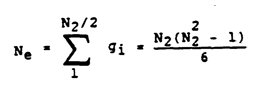
Note that coherent addition is allowable only over four symbol intervals. Then, to avoid excessive computational requirements from frequency resolution that is too fine, the total observation interval of T = NT_S can be broken into N_E blocks of length T₁ = N₁T_s each, where N₁ - 4. Coherent addition is obtained over each of the N₂ = N/4 blocks to compute N₂ envelopes, which are then summed. The latter sum is incoherent addition, but the total S/N is almost the same as for coherent addition over the entire interval T if the individual S/N of each block of four modulation symbol intervals is sufficiently high, such as 10 dB or greater. Therefore, coarse frequency may be acquired with approximately the same probabilities, P₁ and P_m, as previously calculated based on coherent addition over T.

ACQUISITION ON A MODULATED TRANSMISSION

Detection of burst presence and coarse frequency acquisition have been analyzed for an unmodulated carrier. Unfortunately, the omission of preamble overhead for synchronization requires coarse frequency to be acquired on a fully modulated or suppressed-carrier transmission burst. Squaring for BPSK and quadrupling for QPSK can be employed as methods of modulation removal that produce unmodulated components at harmonics of the carrier frequency, f_c. It is these components at 2f_c for BPSK and at 4f_c for QPSK that are used for frequency acquisition. Note that signal squaring for BPSK is equivalent to frequency doubling. Similarly, quadrupling of a QPSK transmission effects frequency multiplication by a factor of four.

There are some problems associated with modulation removal that make frequency acquisition on a modulated carrier considerably more difficult than acquisition on an unmodulated carrier. First, there is an irrecoverable loss in S/N caused by cross-products of signal and noise in the nonlinear processes of squaring and quadrupling. This loss in S/N is very large if the input S/N is low. Such a low input S/N will be the case when the frequency uncertainty F is much larger than the modulation symbol rate, R_s. A second problem with modulation removal is that there will be some other extraneous tones about the desired harmonic. These extraneous tones come from the effect of bandlimiting of the transmitted signal. Because of the extra tones after modulation removal, there is an increased probability of error in the estimation of coarse frequency. Perhaps the worst problem with the process of modulation removal is the expansion of the frequency range, by a factor of two for squaring and a factor of four for quadrupling.

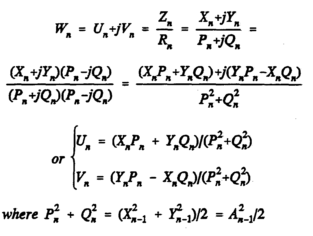
Frequency acquisition is obtained by processing of a complex baseband signal, R = P + jQ. This baseband signal is obtained from quadrature correlators with a reference frequency, f_o, at the center of the band of width F_t = F + B_o. where

F = the total range of carrier frequency uncertainty B_o = the occupied bandwidth of the BPSK or QPSK

transmission.

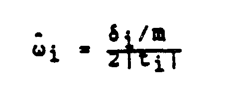
Low-pass filtering with a cutoff frequency of F/2 Hz is employed on the quadrature components prior to sampling and analog-to-digital (A/D) conversion to obtain the P + Q values. Figure 4 depicts the method used to provide the discrete digital signal, R_n = P_n + jQ_n, where n denotes the nth sample. Processing of R_n samples to obtain coarse frequency acquisition is illustrated in Figure 7. Representation of the low-pass signal R over a frequency range of F_t Hz requires s complex samples of R = p + jQ per modulation symbol interval, where F_t = sR_s. With an mth-power operation used for m-ary PSK modulation removal, the sampling rate must be increased by a factor of m to represent an expanded frequency range of mF Hz. The additional samples can be obtained either from interpolation of samples taken at a rate of s per symbol interval, or by increasing the initial sampling rate to provide ms samples of R per symbol interval. It is desired for the signal to be band-limited prior to modulation removal so as to increase the S/N. The bandwidth should be sufficient, however, to avoid significant signal distortion. Hence, a bandwidth of B = 2R_s is chosen. If s > 2 so that F > 2R_s, then the signal at each frequency, f_i = ω_i /2T from f_o, must be filtered to give this bandwidth restriction B = 2R_s.

Before filtering, the signal projection at f_o + f_i is obtained from the complex sample R = P + jQ at multiplier 701. This signal projection will be designated as z = x + jy, where for the nth sample: z_n = R_ne^+jωi^nto or x_n = P_n cos(ω _int_o) - Q_n sin (ω_int_o) y_n = Q_n cos(ω _int_o) + P_n sin (ω_int_o)

In this terminology, t_o is the time interval between samples and is the inverse of the increased sampling rate. 7

Next, recursive filtering of x_n and y_n by filter 702 are employed to impose a low-pass noise bandwidth of B_L = R_s, corresponding to a bandpass noise bandwidth of B_N = 2R_S. For this filtering with a time constant τ , the outputs are designated by X_n and

Y_n.

X_n = e^-t o^{/ τ} X_n-1+(1-e^-to/τ)x_n-1 Y_n = e^-t o^{/ τ} X_n-1+(1-e^-to/τ)y_n-1

For the desired noise bandwidth of B_N = 2R_S,

Thus, the damping factor for the exponential is:

A vector Z_n is defined by the components X_n and Y_n. For m-ary PSK, modulation removal consists of taking the mth power of Z_n at the block 703 to obtain a new vector, w_n, where Z_n = X_n + jY_n

and

W_n = u_n + jv_n

The components u and v for the vector w represent the quadrature components at the mth harmonic of f_o + f_i. In the simplest case of BPSK or m = 2, squaring yields the following components at 2f_o + 2f_i: u =

n

v_n = 2 X_n Y_n

For m = 4, quadrupling for QPSK modulation removal yields components at 4f_o + 4f_i

=

At each frequency in the range of uncertainty F_t, the energy must be computed over the same interval, T = NTs-, of some N modulation symbols. Actually, the range of frequency uncertainty is expanded for BPSK by squaring to 2F_t, and quadrupling for QPSK expands the frequency range to 4F_t. This expansion of the range of frequency uncertainty similarly expands the number of tones at which the energy calculations must be made for determining burst presence and coarse frequency.

Frequency resolution is inversely related to the interval over which coherent addition is performed before the energy computation is made. It is desirable to estimate carrier frequency coarsely in the initial frequency acquisition, in order to reduce the number of tones at which the energy computations are performed. Thus, the total observation interval of T = NT_s should be broken up into some N₂ = N/N₁ sets of length N₁ symbol intervals each, where coherent addition is over the shortened intervals of T₁ = N₁T_s. The envelopes of the N₂ blocks would then be computed and summed to yield the total envelope in each frequency cell. Energy in the frequency cell is proportional to the square of the total envelope.

Squaring loses 6-dB S/N, plus an additional "squaring loss" that is significant only at low E_s/N_o. As shown in (F.M. Gardner, Phaselock Techniques, New York: John Wiley and Sons, Second Edition, 1979, p. 227.), the loss factor is given by: ν₂ = [1 + ( 2E_s/H_o ) ^{- 1} (R_S/B_N)^-1]^-1

With the noise bandwidth of B_N = 2R_S prior to squaring, the S/N loss for BPSK modulation removal is: ν₂ = [1 + (E_S/N_O)^-1]^-1

For reasonable S/N in the intervals T₁ = N₁T_s over which coherent addition is employed, a minimum value of N₁ = 4 symbol intervals is chosen. Consequently, the spacing of the frequency cells will be: 1

With this spacing, the maximum error in location of the closest frequency cell to the location of the second harmonic of the carrier is: δ_max= Δ/2 =

The expanded scale of frequency uncertainty is: F₂ = 2F = 2(F/R_s)R_s = 2sR_s

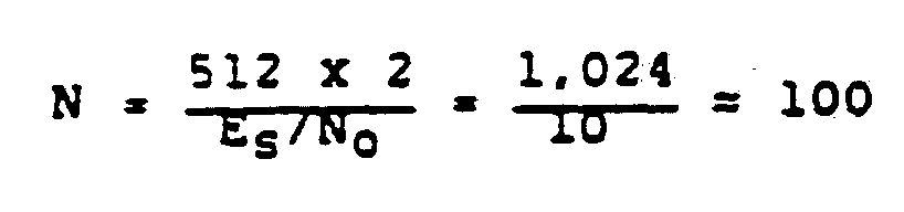
It follows that a total of M₂ = 16s frequency cells are necessary for coarse frequency estimation of a modulated BPSK carrier. If F = 4R_S or s = 4, the required number of frequency cells is seen to be quite large.

M₂ = 16s = 64

With quadrupling for QPSK modulation removal, there is a 12-dB loss in S/N, plus a "quadrupling loss." The total loss factor for quadrupling is given in (J.J. Stiffler, Theory of Synchronous Communications, Englewood Cliffs, New Jersey: Prentice-Hall, 1971, p. 247) by: ν₄ = _j - [1 + 4.5λ.+ 6λ² + 1.5λ³] ^-1

where for B_N = 2R_s,

With two bits per symbol, QPSK would ordinarily have a 3 dB higher value for E_s /N_o than does BPSK. However, the quadrupling causes at least 6 dB more loss in S/N than squaring. Therefore, N₁ = 8 is selected as the minimum number of symbol intervals for coherent addition of the quadrupled QPSK signal. It follows that the spacing of frequency cells will be:

Then, the maximum error in frequency between the closest frequency cell and the fourth harmonic of the carrier is: δ_max = Δ/2 =

Also, the expanded range of frequency uncertainty of the quadrupled signal is:

F₄ = 4F = 4(F/R_s)R_s = 4sR_s

Therefore, M₄ = 64s frequency cells are required for coarse frequency estimation of a modulated QPSK carrier. If F = 4R_s or s = 4, the total number of required frequency cells is:

M₄ = 64S = 256 Note that QPSK requires four times the number of frequency cells as BPSK.

Now consider how the coherent addition is performed by filter 704 over each successive interval of N₁ symbols. For this summation, define the following vector:

W = U + jv

Then, the sum may be updated iteratively to include the last k = msN₁ samples of a sliding block.

U_n = U_n-1 + u_n -u_n-k

V_n = U_n-1 + v_n -v_n._k

The recursive expression of the vector W is as follows:

W_n = U_n + jV_n = W_n-1 + w_n -w_n-k

With a total observation interval of N = N₁N₂ symbols, the vectors W must be converted by block 705 to envelope values for N₂ blocks of symbols and summed. Define:

Finally, the total envelope sum, r_n, over N₂ blocks is updated iteratively as follows: г_n = г_n-k + γ_n The square of г_n is an energy measure for a sliding block of msN samples that includes N = N₁N₂ symbol intervals.

Burst presence is declared when the square of г_n for any of M frequency cells exceeds the energy threshold, E_t. Equivalently, the metric threshold is some value V_t =

Coarse frequency is based upon selecting the frequency cell at which the threshold is exceeded. If the metric threshold is met for more than one frequency cell, the frequency choice is based upon the cell with the greatest value of г_n. Also, the time location at which the maximum metric value occurs yields coarse burst synchronization.

Let E_m/N_o represent the lowest E_s/N_o at which very reliable determinations of burst presence and coarse frequency are required. With mth-order modulation removal, the total S/N in the observation interval of N modulation symbols is:

Ψ = Nν E_m/N_o = N₂(N₁v E_m/N_o)

Here, the loss factor, v , is inversely related to m², where mth-order multiplication is used for m-ary PSK modulation removal. Note that m = 2 for BPSK and m = 4 for QPSK. The block length is N- = 2m, which has a value of 4 for BPSK and 8 for QPSK. It will be assumed that:

It follows that for both BPSK and QPSK, N₁ ( νΕ_m /N_o) = ( 2m) (2/m) = 4 and the total S/N in the observation interval T = NT_s is therefore related to the number, N₂, of blocks by: ψ = 4N₂

Optimum energy thresholds will be assumed separately for BPSK and QPSK, based upon the E_s/N_o values at which νΕ_m/N_o = 2/m. With these optimum thresholds, the probability. P₁, that noise can cause false detection in a given time-frequency cell and the probability P_m of missed detection on the signal are approximated as:

P₁ = ^e-0.25ψ = e^-N2

P_m = Φ

P_m is smaller than P₁ by one order of magnitude. Thus, the important consideration for UW performance is how large does the observation interval N = N₁N₂ in modulation symbol intervals have to be to yield a desired P₁. Table 4-1 gives required values of N₂ and N for BPSK and QPSK as a function of the required P₁. In general, the P₁ values are expressed as:

P₁ = 10^-1 where I is a positive integer. It follows that the required number, N₂, of blocks of length N, is given by:

N₂ = I In 10 = 2.3 I Also, a total observation interval of N symbols is required, where

{ 9.21 for BPSK

N = N₁N₂ = 2mN₂ = 4.61m =

{ 18.41 for QPSK

Omission of the synchronization preamble for improving the access efficiency implies that the message bursts are not very long. The burst length places an upper bound on the available observation interval for coarse frequency acquisition. From Table 4-1 it is seen that large observation intervals, N (measured in modulation symbols), are required if the probability, P₁ , of false detection is to be very low.

For instance, a P₁ = 10^-8 specification necessitates N = 72 for BPSK and N = 144 for QPSK. It appears that the requirements on N may be too severe for QPSK unless the specification on P₁ is relaxed considerably. An alternative method of burst detection and frequency acquisition will be investigated next that avoids quadrupling for modulation removal and the consequent large requirement on N.

Table 4-1. Required Observation Interval for a

Specified Performance in False Detection

of Burst Presence

The P₁ and P_f computations were based upon all of the energy after m-order modulation removal being in an unmodulated tone at mf_c. Such would be the case if the pulse shapes were rectangular. In the most critical cases for frequency acquisition where F » R_s, the symbol rate, R_s, is low. Bandwidth efficiency is then of only minor concern, and the transmitted pulses could be approximately rectangular. Light filtering prior to squaring or quadrupling will give some pulse distortion and result in some energy at locations other than mf_c. For BPSK or m = 2, the bandwidth restriction is manifested solely as envelope distortion. Therefore, hard limiting of the envelope either before or after squaring would yield, a squared output only at 2f_c

For QPSK, the effect of band-limiting is conveyed primarily by a gradual phase shift when there is a 90° transition. Consequently, there will be some energy at other than 4f_c after quadrupling. even if the envelope is limited to a constant value, Thus, the extraneous tones would cause some increased probability of incorrect estimation of coarse frequency for QPSK. The effect is minimized by avoiding any significant filtering prior to quadrupling.

Alternative Method of Frequency Acquisition

In the method just analyzed for detecting burst presence and estimating coarse frequency, UW detection is not required until coarse frequency is acquired. Consequently, UW detection need be performed for one frequency location. In the case of QPSK, however, the quadrupling for modulation removal resulted in the requirement of energy measurements for a very large number of frequency cells. Furthermore, the required observation interval for reliable frequency estimation was very long, more than may be available in a burst duration. An alternative method of acquiring coarse frequency that includes UW detection will now be described. This recommended method reduces the required number of frequency cells for estimating coarse frequency at the expense of UW detection on all of these cells.

Knowledge of the UW pattern allows modulation removal in a form similar to decision feedback (DFB) of modulation decisions. Thus, the vectors, Z_n, are multiplied by a known vector sequence in place of squaring or quadrupling. Multiplication of the signal by the known UW pattern does not expand the frequency scale or require an increased sampling rate, as does squaring and quadrupling. It follows that the number of frequency cells required for estimating coarse frequency is reduced by avoiding either squaring or quadrupling. Even if the message burst utilizes QPSK modulation, the UW may be binary by using only two antipodal vectors of the QPSK constellation. With the binary UW, modulation removal is effected by convolution of the discrete signal for each frequency cell with a known UW sequence of +1 and -1 values.

In the previous algorithm for coarse frequency acquisition, an mth-power operation was employed for M-ary PSK modulation removal: squaring for BPSK and quadrupling for QPSK. Taking the mth power of the complex signal expands the phase angles by a factor of m, thereby decreasing the S/N by a factor m². Moreover, this nonlinear technique of modulation removal yields second-order noise terms from cross products of signal plus noise. The additional noise power is related to the bandwidth prior to modulation removal. Because of a large frequency uncertainty of F in addition to the signal bandwidth occupancy of B₀, the initial frequency band has a width of F_t = B_o + F. Therefore, it was necessary to filter at each tone of the coarse frequency representation to a bandwidth close to B_o prior to modulation removal in order to minimize the additional noise. Such prefiltering is not required when the UW itself is used as a multiplier for modulation removal.

Multiplication of the signal at each tone by the UW effects modulation removal only near the correct time/frequency locations. The operation is linear, however, and the phase angle is not magnified by the process. Thus, there is no loss factor of m for the S/N. Also, the linear operation does not cause any second-order noise terms. Consequently, filtering prior to modulation removal is unnecessary. Matched filtering must be employed at some point to maximize the S/N at the detection instants for bit decisions. Such matched filtering need be performed only for the winning tone in coarse frequency acquisition. Therefore,* filtering requirements are reduced by avoiding filtering prior to modulation removal and performing matched filtering after coarse frequency is acquired.

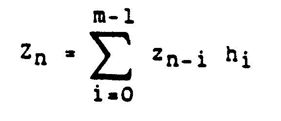
As for the previous technique, the complex samples z_n = x_n + jy_n for each frequency cell could undergo recursive filtering at filter 702 to produce samples Z_n = X_n + jY_n that have a bandwidth constraint of B_n = 2R_S. It is the vector Z_n that must be convolved with the UW pattern to obtain an envelope at each frequency cell. It is recommended, however, that this filtering be omitted, in which case the vector Z_n is identical to z_n. Because the total frequency range of F_t = sR_s requires s complex samples per modulation symbol interval T_s = 1/R_s, the binary elements of the UW must be repeated s times. With this definition of the expanded UW represented by elements h_n, the output, W_n, of the convolution yields:

W_n = Z_n Z_n-1

Note that the total observation interval of T = NT_s now corresponds to a UW length of N, measured in modulation symbol intervals. Because of the repetition of sample values, the expanded UW contains N_e = sN elements. The interval, T, must span a sufficient number, N, of symbols to yield the desired performance in terms of P_m and P_f. The required length N is smaller than when mth-order modulation removal is employed, because multiplication with the known UW sequence does not reduce the S/N.

It is desirable to keep the frequency resolution as coarse as possible to reduce the number of frequency cells. The resolution must be sufficient, however, to allow matched filtering on the samples after the coarse frequency correction is made. Thus, coherent addition should be restricted to the shortest interval that yields a high S/N and yields adequate resolution for matched filtering. This restriction means that straight convolution cannot be employed. Instead, the length, N, must be grouped into N₂ blocks of N₁ symbols each. Because the decision removal of modulation does not cause a loss of S/N, N₁ = 2 might suffice for coherent addition. Adequate resolution for performing matched filtering after frequency correction makes N₁ ≥ 4 necessary, however. Thus, coherent addition will be over an interval of N₁ = 4 modulation symbols or k = 4s complex samples. Then, there will be N₂ = N/4 blocks of k samples each.

Now define the convolution over the shortened interval of four modulation symbols or k = 4s samples for the nth block by:

E_n = Z_nk-i h_i

In terms of quadrature components.

W_n = U_n + jVn where.

The vector W_n is used to form a noncoherent metric, γ_n.

For each frequency cell, the total metric г_n for the observation interval of N symbols is the sum of γ_n values for the N₂ blocks.

False detection of a burst presence can be caused only by noise. Although the UW may be falsely detected before it is in the correct time location, use of a suitable UW will yield a larger correlation when the alignment is achieved. A UW pattern should be chosen that has low autocorrelation for all time displacements relative to the correlation when aligned. Then, maximum correlation should occur at worst only a sample or two away from correct time alignment. With such resolution of a fraction of a modulation symbol interval in coarse burst synchronization, fine burst alignment will be obtained when symbol synchronization is acquired on the output of the matched filter. It is assumed that there will be no time overlap of transmission bursts. Also, the burst length will be known. Therefore, the receiving station will have acquired any previous burst and know where that burst ends. Consequently, the memory of the energy measures for the M frequency cells can be zeroed prior to arrival of the new burst. This memory erasure prevents problems of false detection of the present burst from energy in the preceding burst.

With the UW appended to the front of the message burst, the message burst cannot cause false detection unless the UW is missed. Therefore, the UW detection for burst presence and estimation of coarse frequency should have a low value of P_m. Note that the pattern of the UW is not very critical for P_m, but the UW pattern must be known and be of sufficient length, N, to provide a low value of P_m. Use of a pseudo-random pattern or a Barker sequence for the UW is necessary to improve its autocorrelation properties so as to make a less coarse resolution of burst time location and yield a low probability P_f of false detection.

It is assumed that the metric threshold for UW detection is based on some minimum value of E_m/N_o for the ratio E_s/N_o of signal energy per modulation symbol to noise power density. With this fixed threshold, false detection in any frequency/time slot will have some constant value that is dependent upon the E_m/N_o upon which the threshold is based. The probability of missed detection in the correct time/frequency cell will be lowered, however, for E_s/N_o values above the minimum of E_m/N_o. Usually, E_m/N_o≥ 4, which means that the S/N per block of N, = 4 symbols would be at least 16. This S/N is sufficiently high so that the use of a noncoherent metric should yield performance almost as good as if coherence were employed over the entire UW rather than over the N, individual blocks, where N = N₁N₂ is the total UW length.

Optimization of the detection threshold is often based upon minimizing the sum P₁ + P_m, where P₁ is the false detection probability at one frequency/time location when the signal is absent, and P_m is the miss probability in the correct frequency/time slot when the signal is present. The UW must have a fairly high S/N, Ψ, in order for reasonably low values of P₁ and P_m to be achieved. For this case of high S/N per word, the optimum threshold is approximately at 0.5 г_s, where г_s is the UW detection value from signal alone with perfect alignments in both frequency and time. For this case of high Ψ, P₁ and P_m may be approximated as follows:

P₁ = e^-0.25Ψ » e^-0.25NEm^/No

where

N = UW length in modulation symbols

E_m./N_o = lowest E_s/N_o for which highly reliable

synchronization is required.

Use of the so-called optimum threshold results in P₁ being one order of magnitude larger than P_f. It is desirable for P₁ to be much smaller than P_m, as will now be explained. Let P_f denote the overall probability of false detection over some M tones and N_a symbol intervals of signal absence prior to burst arrival. It is reasonable for the threshold to be set to balance P_f and P_m. The total probability of false detection may be approximated by its union bound of:

P_f ≈ MN_aP₁

Adjustment of the UW detection threshold to balance P_f and P_m can be achieved by increasing the threshold above 0.5 T_s. Assuming that MN_a might be as large as 10³, a detection threshold Of V_t =

г_s may be appropriate. With this threshold, probabilities of false detection and missed detection can be approximated as:

P_f = MN_ae^-0.3Ψ = MN_ae^-0.3NEm^/No m

For the purposes of computing P_f and P_m values and determining the required UW length N, the minimum value of E_s/N_o under consideration will be chosen as E_m/N_o = 4. Because of the close spacing of the M tones for coarse frequency estimation, the effective number of independent tones will be much smaller than M. It will be assumed that the effective number of independent time/frequency values is N_e = 100, which may be considerably smaller than the product MN_a. With these assumptions, use of a detection threshold of V_t

Γ_s yields a reasonable balancing of P_f and P_m.

UW detection probabilities are then approximated by the following two expressions: P_f =N_ee^{-0.3 NE}m^/No = 100 e^-1.2N

P_m - Φ[/2(0.2 NE_m/N_o)] = Φ[√2(0.8 N)]

Table 4-2 gives P₁ and P_m values as a function of UW length N. A length of N = 16 may be adequate for reliable detection of burst presence and the estimation of coarse frequency. There is a valid argument, however, for the use of a larger N, such as 24. Modulation removal is necessary for carrier synchronization, the estimation of fine frequency and carrier phase. If the UW is of length N = 24, then the total S/N in the UW will be high enough for accurate estimations of these carrier synchronization functions. The pattern removal of the UW serves as modulation removal, so that the necessity of squaring is avoided. Removal of the known UW pattern, therefore, improves the performance of carrier synchronization because it does not lower the S/N as does squaring and quadrupling. Multiplication of the signal with its delayed replica is necessary in symbol synchronization rather than pattern removal. Use of a pseudorandom UW with N/2 transitions provides a good pattern for reliable symbol synchronization.

In UW detection for burst presence and coarse frequency estimation, the detection threshold could be exceeded when there are small errors in both time and frequency. Therefore, the time/frequency accuracy of detection is improved by selecting the combination of time and frequency cells that yields the largest metric. Furthermore, coarse burst synchronization is based upon the time location of the maximum metric. Therefore, continued metric determinations and metric comparisons should be performed over frequency and time for an interval of one UW length after the initial detection of burst presence.

Table 4-2. Detection Probabilities for

Burst Presence and Coarse Frequency

Estimation as a Function

of UW Length

* Based upon a m n mum E_s/N_o of E_m/N_o = 4

and the assumption of P_f = 100 P₁.

It has been assumed in the preceding calculations that the UW detection threshold was a fixed value based upon some E_m/N_o, the minimum value of E_s/N_o for which highly reliable synchronization is required. With this fixed threshold, the false detection probability, P₁, for any frequency/time cell during signal absence is a constant. As E_s/N_o increases above its minimum value, however, the miss probability in the correct frequency/time cell is lowered dramatically. Thus, P_m becomes much smaller than P_f when E /N is several dB above the assumed minimum.

Previous transmission bursts from the same source may be monitored to estimate the received signal level. With such estimation of received signal level, an adaptive UW threshold can be employed. The adaptive threshold would be related to the signal energy level per symbol, E_s. Hence, P_f and P_m would both be decreased with increasing E_s/N_o, and remain fairly balanced at all signal levels.

If previous bursts are not used for signal level estimation, then any adaptive UW threshold must be based upon the level of the present reception. When the signal is absent, the detection threshold is therefore based upon noise energy. Consequently, P, and P_f = N_eP₁ will be constants irrespective of E_s/N_o. This adaptive threshold technique is termed CFAR for "constant false alarm rate." When the signal is present the energy estimation is based upon signal plus noise. Thus, the detection threshold is increased with signal energy, so that P_m only has a moderate decrease as E_s/N_o is increased.

UW SELECTION

In terms of false detection probability, P_f, when the signal is absent and missed detection probability, P_m, when the signal is present, UW performance is dependent upon word length N, but is the same for any UW sequence. Thus, the UW sequence would not be critical if the detection of signal absence or presence was all that was required. The maximum absolute value of correlation over frequency and time is used, however, to provide both coarse frequency estimation and coarse burst synchronization. It is necessary for the timing error in coarse burst locations to be less than one-half of a symbol interval of correct alignment. With this accuracy in coarse alignment available, perfect burst synchronization is then achieved by the acquisition of symbol synchronization after matched filtering. Therefore, a UW sequence must be employed that has autocorrelation properties which provide the necessary resolution of burst time.

A UW pattern must be chosen that has very low autocorrelation for any time displacement from correct alignment. Use of a sampling rate of f_s = sR_s results in s complex samples per modulation symbol interval. With a UW that has low autocorrelation for any number of symbol intervals of timing error, there are still 2s - 1 positions of partial or complete UW alignment that can yield fairly large correlations. The correlation peaks for perfect alignment, and falls off for adjacent samples on either side of perfect alignment. For E_s/N_o values of interest, coarse burst synchronization will therefore almost always be either correct or only in error by ±1 sample interval.

Autocorrelation for the UW is proportional to the difference between the number, N_A, of agreements and the number, N_D, of disagreements. For perfect time alignment of the received UW and its stored replica, there are either all N agreements or all disagreements, and the metric based on absolute values would be г = | N_A - N_D | = N. Prior to time alignment by δ symbol intervals, only the first N - δ symbols of the UW word would have arrived. In the correlation process, the first N - δ received symbols would be compared to the last N - δ symbols of the stored UW replica. In the other δ locations for symbols in the correlation, δ received symbol intervals of noise only prior to UW arrival would be correlated with the firstδ symbols of the stored UW replica. In order to reduce the number, M, of required frequency cells for coarse frequency estimation, the frequency resolution is set to be adequate for coherent addition or pure correlation over only N₁ = 4 modulation symbol intervals. Thus, the UW of length N = N₁N₂ is processed as N₂ separate blocks of length N₁ each, and noncoherent addition is employed to combine the separate correlations for the N₂ blocks. The shortened correlation intervals and noncoherent combining make the UW sequence selection more difficult for achieving the desirable autocorrelation properties. Low overall metrics for the UW detection must be achieved for any timing error of one or more symbol intervals.

A recommended UW of length N = 16 is listed in Table 4-3. Also, its autocorrelation metrics for different time displacements, δ , are given for two cases. First, the metrics for the case of interest are tabulated, where individual correlation metrics (γ_0, γ₁, γ₂, γ₃) over N₁ = 4 symbols are made for N₂ = 4 blocks and then combined noncoherently. Second, metrics based upon correlation or coherent addition over the entire UW length N = N₁N₂ are given as a reference. The total metric values for this UW choice are not greatly affected by the restricted correlation interval of N₁ = 4 symbols and noncoherent addition of the N₂ = 4 block metrics. In both cases, the maximum metric of г_s = 16 is achieved with perfect alignment, δ = 0. An error in alignment of δ = 1 also yields the largest metric for any non-zero time displacement, and this value is г = 5 for both cases. Thus, use of this UW appears to overcome the handicap of restricted coherent addition over only N₁ = 4 symbol intervals and noncoherent combining of the N₂ = 4 block metrics of γ_0, γ₁, γ₂, γ₃and γ₃. Also, from Table 4-2, a UW of length N = 16 yields low values of P_f and P_m, even when the detection threshold is based upon a minimum E_s/N_o as low as E_m/N_o - 4. Therefore, this UW appears to be a good choice for most applications.

Table 4-3. Recommended UW Sequence*

and its Autocorrelation Metrics

*UW of Length N = 16: 0000 1100 1100 1111

**г = |lγ_i|

MATCHED F ILTERING AND SAMPLE INTE RPOLATION

After coarse frequency acquisition, the stored complex signal will have some small residual frequency error, f. Because the spacing Δ of the correlation tones for estimating coarse frequency is less than or equal to one-eighth of the modulation symbol rate, R_s, I it follows that

|f| ≤ R_s/16 when the correct coarse frequency is selected. With such a small error in frequency, matched filtering can be employed prior to other demodulator processing.

The discrete signal has s complex samples per symbol, corresponding to a digital sampling rate of f_s = sR_s. Usually, s = 4 will be adequate to represent the total band of width B_t = B_o + F, where B_o is the occupied bandwidth of the signal and F is the range of frequency uncertainty for the carrier location. Matched filtering of this discrete signal is performed, and the filter output at the same sampling rate of f_s = sR_s is the input to the symbol synchronizer.

Processing of the filtered samples by the symbol synchronizer yields an estimate of the desired sampling times for bit detection. Only one complex sample per symbol is used in processing after symbol synchronization. These sample values must be obtained from the output of the matched filter by interpolation that yields one complex sample per modulation symbol interval at the timing location obtained from symbol synchronization. Both matched filtering and sample interpolation will be examined in this section of the disclosure.

There are three basic types of digital filter implementations. First, there is direct convolution, which is suitable only for filtering that can be represented by a finite impulse response (FIR filters). Second, a recursive implementation may be employed for any filter response associated with "poles" and "zeros." The third method is so-called "fast convolution," in which fast Fourier transforms (FFTs) are employed to perform filtering based upon a frequency domain representation of the filter function. All three of these implementations of digital filters are discussed in (B. Gold and CM. Rader, Digital Processing of signals, New York: McGraw-Hill Book Company, 1969).

It is possible to use the same filter module for matched filtering and interpolation. The total computation is simplified, however, by separate filters for the two functions. Therefore, matched filtering will be performed first, with a complex sample rate of f_s = sR_s for both the input and the output of the matched filter. Processing of the output samples from matched filtering is performed then by the symbol synchronizer, which derives a timing phase estimate. Use of this timing phase for a clock at the symbol rate of R_s determines the one appropriate sample time for bit detection during each symbol interval. A second filter is then employed for interpolation. The output of the matched filter constitutes the input to the interpolation filter. Outputs for the interpolation filter are computed only at the sampling instants (one per symbol) defined by the timing phase from the symbol synchronizer. Figure 8 depicts the configurations of matched filtering by block 801, symbol synchronization by block 803, and sample interpolation by block 802. Overall Nyquist filtering, as described in the Lucky et al reference discussed above, is desired so that no intersymbol interference (ISI) occurs at the detection sampling instants. With matched filtering at the receiver to maximize the S/N at detection sampling instants, the total Nyquist response is separated into a square-root Nyquist response for the transmit filter and the same response at the receiver. In order not to change the overall response, the interpolation filter has a flat response over the signal bandwidth, and the amplitude then rolls off gradually to zero before the end points of ±f_s/2 for the sampling spectrum. The interpolation process could be considered as an inherent part of symbol synchronization, but interpolation will be treated here as a separate process associated with filtering after a timing estimate is provided by the symbol synchronizer.

MATCHED FILTERING

Matched filtering with a square-root Nyquist function has an infinite impulse response. Use of only the significant portion of the impulse allows an FIR implementation using direct convolution. Truncation of the impulse response does cause some spectral distortion, but this distortion is very small if most of the energy is conveyed by the finite portion of the impulse response that remains after truncation. Also, the impulse response should be truncated equally to both sides of its main time lobe, so as to have symmetry about the point of mean delay. Such symmetry avoids delay distortion.

Recursive implementation of digital filtering is appropriate when the filter response is based upon the poles and zeros of the frequency response function. Although the square-root Nyquist response ideally has no delay distortion,, it can be approximated by designs based on poles and zeros of the transfer function. Locations of poles and zeros are given in (J.J. Poklemba, "Pole-Zero Approximations for the Raised Cosine Filter Family," COMSAT Technical Review, Vol. 17, No. 1, pp. 127-157) for excellent approximations to square-root Nyquist filters of various rolloff factors from 0.1 up to 1.0. Hence, recursive techniques may be employed for digital implementation of these filter designs. The recursive implementation yields an output that is impulse invariant with respect to the analog filter function. For a filter with some M_p poles and M_o zeros, the recursive representation of filtering yields an output, Z, as a function of input z in accordance with the following equation:

where a_i and b_i are coefficients that for a given sampling rate yield the desired response.

A total Nyquist frequency response with a rolloff factor of p would ideally have flat delay over the entire band and flat amplitude out to ±(1 - ρ)R_s/2 from band center. The rolloff of amplitude has skew symmetry about ±R_s/2, with total cutoff occurring at ±(1 + ρ)R_s/2 from band center. Thus, the total bandwidth for non-zero amplitude is R_s (1 + ρ). The minimum bandwidth for a "brick-wall" Nyquist response is R_s, corresponding to ρ = o, and the total bandwidth increases proportionally with p. Therefore, the rolloff factor p is also referred to as the fractional excess bandwidth. The low-pass amplitude response (that for positive frequencies) is given for cosinusoidal rolloffs by

1 for O ≤ f ≤ f_a

A(f) - ( 0.5 + 0.5 cos π for f_a ≤ f ≤ f_b

₀

for f > f_b where

f_a = 0.5 R_s (1 - ρ) f_b = 0.5 R_s (1 + ρ)

Such a Nyquist function in the frequency domain results in a time domain waveform that has zero crossings at intervals of ±nT_s about pulse center. Consequently, use of a pulse or symbol rate of R_s = 1/T_S yields nulls of all other pulses at the center of any one pulse. This property of ISI nulls is the main feature of Nyquist signaling. The full Nyquist pulse shape may be defined about its center at t = 0 by

i

Figures 9a and 9b give plots of Nyquist frequency responses and impulse responses, respectively, for different rolloff factors of ρ = 0.0, 0.5, and 1.0. The corresponding pulse shapes are also shown. Whereas decreasing the rolloff factor reduces the signal bandwidth, the time interval of significant pulse level increases for decreasing ρ. Small timing errors will result in too much ISI at detection sampling points if ρ < 0.2. As seen from the preceding equation the range of significant pulse amplitudes includes only the main lobe and two time sidelobes on each side of the main lobe when ρ = 0.5. Therefore, the filter response for ρ ≥ 0.5 can be closely approximated as an FIR filter with a finite impulse response of width 6T_s. For such a filter with some m terms included in the impulse response, h_i, finite convolution is represented mathematically as

A very simple filter may be used to approximate a square-root Nyquist filter with a rolloff factor of p = 0.4. This approximation consists of a delay- equalized four-pole Butterworth response that has a 3- dB cutoff at ±0.5 R_s about band center. The poles for a Butterworth filter are spaced at equal angles symmetrically about the real axis in the left-half plane of the complex frequency representation. As seen from Figure 10, all poles lie along a circle of radius r = 0.5 R_s from the origin of the complex frequency scale. A simple delay equalization is provided by a single pole/zero pair on the real axis at distances of ±1.2 (0.5 R_s) from the origin. Although such a simple filcer does not yield a nice symmetrical pulse, the ISI at sampling instants for two such filters in tandem is very small and results in a performance loss of only about 0.2 dB, even at bit error probabilities as low as P_b = 10^-7 when the modulation is either BPSK or QPSK. This useful filter may be readily implemented using the recursive technique. One advantage to use of a truncated impulse response and direct convolution is that the filter is represented exactly over the finite region. The amplitude function of frequency for a square-root Nyquist approximation is then completely symmetrical, and there is no delay distortion. Consequently, ISI will be zero at the correct sampling instants for bit decisions. For a sampling rate of f_s = sR_s with s = 4 samples per symbol, note that an impulse response of only 25 terms is required to represent a truncated response of width 6T_s. This implementation of direct convolution to approximate a square-foot Nyquist response with p = 0.5 is recommended.

SAMPLE INTERPOLATION

Sample interpolation is simplified by the use of a filter with a finite impulse response of short duration and implementation by direct convolution. In order to have a short impulse response, the filter must have a bandwidth considerably wider than the signal spectrum. This requirement is easily met by extending the passband to ±2R_S about band center, where f_s = sR_s is the complex sampling rate and there are s > 4 samples per modulation symbol interval, T_s. Even if the modem filtering had a rolloff factor of ρ = 1.0 for the tandem of two square-root Nyquist filters, the signal spectrum would still be contained in a region within ±R_s of band center. It is assumed here, however, that ρ = 0.5 is employed for the modem filters. Another requirement on the interpolation filter is for its amplitude to be flat over the signal spectrum. A filter that satisfies the two requirements for the interpolation process is one with a full Nyquist response, a rolloff factor of ρ = 1/3, and a location of ±1.5R_s about band center for the 6-dB attenuation or half-amplitude points. Although the impulse response is not truly finite, truncation of the impulse response to only its main lobe and two sidelobes on each side will convey all the significant response. With its mean delay represented at the delay origin, the impulse response for this interpolation filter is expressed as

In this expression, T₁ = 1/B₁ is the "Nyquist" interval for this interpolation filter—the pulse interval that would produce samples without ISI. B₁ is the Nyquist bandwidth between the two half-amplitude points, as

B₁ = 2(1.5R_s) = 3R_s

Thus,

It is possible to reuse the matched filter for interpolation. In such a case, the output of the matched filter would be computed once per symbol interval as a function of its input, which has four or more samples per symbol interval. Because the matched filter has a narrower bandwidth than the response just proposed, the width of the impulse response measured in symbol intervals must be increased, which requires more terms to represent the truncated impulse response. Therefore, it is recommended that a separate filter following matched filtering be employed for interpolation. The impulse response just discussed, which is based on B₁ = 3R_S and ρ = 1/3, is a suggested choice for the interpolation filter. The output of the matched filter at s ≥ 4 complex samples per symbol constitutes the input to the interpolation filter. In accordance with the timing estimate from the symbol synchronizer, one output complex sample per symbol is computed for the interpolation filter.

Quadrature timing references with frequencies of R_s and some arbitrary phase delay of ξ are used to obtain correlations U and V with the envelope squared of the samples from the matched filter. These correlations are used by the symbol synchronizer to obtain an estimate β of the actual signal timing phase and the amount λ by which the delay of the reference timing should be increased. The required additional delay is the difference between

and ξ, as

ξ

It is assumed that the input to the filter has s=4 complex samples per symbol interval. After symbol synchronization is acquired, the s=4 complex samples for the nth symbol interval have time subscripts of 4n, 4n+l, 4n+2, and 4n+3. There is a timing offset of 0.5T, where T = T_s/4, relative to the sample subscript. Thus, sample 4n lies at 4nT + 0.5T, or 0.5T from the symbol boundary. If

= 0, the one sample per symbol would be calculated for the output of the interpolation filter at time instants of 4nT + 2.0T, where T = T_s/4 is the interval between input samples. Thus, for no error in reference timing (

λ = 0), the output complex samples of the interpolation filter would be defined in terms of its truncated impulse response by a center term and some number, n₁, of terms to the left and right of center. Z(4nT + 2.07) = h(kT + 0.57) z (4nT * 1.5T - kT)

Here, z denotes the input sample values and Z the output values for the interpolation filter. The truncated impulse response is represented relative to its mean delay so that h(iT) is symmetrical about its relative delay origin.

With h(kT) truncated to two time sidelobes on each side of the main lobe, the impulse response is defined from -3T₁ to +3T₁. But T₁ = (4/3)T, so the interval is from -4T to +4T. Thus, n₁ = 4, and the implementation of FIR convolution is equivalent to the use of a tapped delay line that has 2n₁ + 1 = 9 taps. The 2n₁ + 1 = 9 tap gains vary, however, as a function of the required timing shift,

.

For digital implementation of filtering,

£ must be quantized into some number m, of input sample intervals of T plus a fraction of T expressed as m₂t_o. Here, the delay t_o represents the resolution for symbol synchronization, which should be perhaps 256 timing steps per modulation symbol interval, or

If there are s = 4 input complex samples per symbol interval, t_o is then 1/64 of the input sampling interval T,.

Symbol synchronization indicates a need for a change λ in timing phase, corresponding to an increased timing delay or t₁, where

This quantity t₁ must be quantized into a linear combination of some number m₁ of steps T plus m₂ steps of t_o. Let t_e represent the quantization error, where

|t_e| ≤ 0.5 t_o

Then, quantization of t₁ results in the following equality: t₁ = m₁T m₂t_o + t_e

For quantization that determines m₁, the quantity

A₁ is defined as

Then, m₁ is the greatest integer, positive or negative, that does not exceed A₁, as given by m₁ = [A_t] After the expression of part of t₁ as m₁T, the residual timing change is termed t₂, where t₂ = t₁ - m₁T

Now, define a quantity A₂ as follows:

The integer m₂ for quantizing into timing steps of t_o is given by the closest integer to A₂, as m₂ = [A₂]

For any given timing position, there are only 2n₁ + 1 = 9 values of h(t) that must be used. The m₁T portion of the timing shift can be effected in the convolution by shifting the time indices of the input samples by m,. The m₂t_o portion of the timing shift must be represented, however, by a shift of delay for the impulse response. There are T/t_o = 16 possible values of m₂, with integers from 0 through 15. Consequently, T/t_o = 16 different sets of the 2n₁ + 1 = 7 values for h(t) must be stored, with one set of 2n, + 1 values of h(t) for each value of m₂. In general, the output of the interpolation filter for a quantized timing shift of m₁T = m₂t_o is given by direct convolution as

Z(4nT + 2.07 + m₁T + m₂t_o) = h(kT + 0.5T + m₂t_o)

z(4nT + 1.5T + m₁ ^T - kT) The interpolation filter provides the signal values at the appropriate time instants (mid-symbol) for bit decisions. This interpolation is necessary in order to process only a few samples per symbol, such as s = 4. If s = 16 were employed, the processing requirements in complexity and speed would be increased, and the interpolation filter would be unnecessary. Instead, symbol synchronization would select for each symbol the sample that was closest to mid-symbol for further processing, including bit decisions.

Symbol Synchronization

Symbol synchronization is investigated for burst communications without the use of preamble overhead for the acquisition of carrier synchronization and symbol synchronization. Overhead is assumed for a unique word (UW) that is necessary to accurately define the starting location for the message portion of the burst. In the above discussion, it was found advisable to utilize the known UW pattern as an aid in the detection of burst presence and the acquisition of coarse frequency. After the acquisition of coarse frequency, matched filtering is implemented as was just described above. The next processing step is to obtain symbol synchronization, which will be described now.

In the determination of burst presence and coarse frequency, use of the UW establishes the burst location approximately. It is assumed that the burst length will be known prior to reception. Therefore, the starting and ending boundaries of the burst should be known after coarse frequency acquisition. Also, burst synchronization after matched filtering is retained either by accounting for the group delay introduced by filtering or by performing UW detection on the output of the filter. It follows that the entire burst (except for a very small guard space for time uncertainty) can be processed to obtain symbol synchronization.

The only signal attributes useful to symbol synchronization are provided from symbol transitions. Usually, the UW has transitions in symbol values exactly one-half of the time. Because these transitions are always present in the UW, the UW can provide a good pattern for acquiring symbol synchronization. The data have an average transition probability of one-half, but can have long intervals without transitions. On the average, the transitions in the data will aid in symbol synchronization. A nonlinear operation (such as squaring) is necessary to obtain symbol synchronization from the complex samples out of the matched filter. The operation can be the same for any portion of the burst, including the UW. Therefore, the UW and the data burst can both be used in obtaining symbol synchronization.

Two modes of synchronization are usually employed in burst communications: acquisition and tracking. In conventional burst communications using synchronization preambles, symbol synchronization is acquired during the preamble. Then the timing estimate is maintained with continued tracking by the symbol synchronizer throughout the data burst following the preamble. When there is no synchronization preamble, either the UW or the entire burst can be used for the acquisition of a coarse timing estimate. Then a second processing of the same burst may be employed to refine the estimate of symbol timing. Thus, fine resolution of symbol timing can be achieved by a two-step processing of the entire burst. This second step in symbol synchronization that is used to obtain a fine timing estate does not constitute a tracking mode of synchronization, but is merely a second step in acquisition.

Although two-step methods of symbol synchronization were investigated, the recommended method achieves a timing estimate in one step, without the necessity of an initial acquisition of coarse frequency. Also, the algorithm is effective for either BPSK or QPSK. This recommended technique is based upon a Fourier spectral component at the modulation symbol rate in the squared envelope of stored complex samples of the demodulated burst. With reasonable restriction of the signal bandwidth to less than twice the symbol rate, a sampling rate of s = 4 complex samples per modulation symbol will suffice for accurate computation of the Fourier components at the frequency of the symbol rate.

It is shown that the rms error of the timing estimate can be reduced to only 2 percent of a modulation symbol interval when the burst length is at least N= 100 symbols and E_s/N_o = 10 dB. With this accuracy in symbol synchronization, the timing jitter will not cause a significant loss in detection performance. The analysis of timing jitter is for continuous signals, but is applicable to the discrete case if the sampling rate is sufficient to derive the Fourier components without distortion from undersampling. Description of Symbol Synchronization

Symbol synchronization is achieved by processing the complex samples obtained from the output of the matched filter. In principle, two complex samples per symbol are adequate to obtain symbol synchronization from a band-limited signal. The algorithms for symbol synchronization can utilize two or more complex samples per symbol interval. It is not known whether the accuracy in symbol synchronization will be sufficient on two samples per symbol unless the timing estimate is further refined by an additional stage of processing of new samples from the matched filter after the first timing correction. Consequently, it may be desirable to use four samples per symbol to avoid the necessity of a repeated stage of synchronization for improving the fine timing estimate.

After symbol synchronization is achieved, whether in one stage or two, the input of the matched filter must be determined for the complex samples at the new timing. In all further processing for carrier synchronization and data detection, the maximum signal-to-noise power ratio (S/N) is achieved for the samples located near the middle of each modulation symbol. In fact, for symmetrical pulses, the optimum sampling point is precisely at midsymbol. Only the one sample per symbol at the midsymbol location should be computed from the output of the matched filter to be used in further processings after symbol synchronization is obtained.

Even if symbol timing is accomplished in one stage of processing, this stage may consist of two steps. The first step is to acquire coarse timing. Coarse timing merely groups the complex samples correctly so that, for a rate of s complex samples per modulation symbol, each group of s samples lies within the same symbol interval. In the second step of symbol synchronization, fine timing is obtained. Fine timing consists of estimating where, between adjacent samples of different symbols, the symbol boundary is located. In the estimations of symbol timing, an average over some number N of symbols is required to reduce the estimation errors introduced by signal disturbances from additive noise and sometimes by intersymbol interference (ISI).

There are many possible algorithms for symbol synchronization that will yield approximately the same performance. Only a few such algorithms will be examined. Some of these algorithms are effective for both BPSK and QPSK modulations. Others are, however, effective only for binary modulations. It should be remembered that a binary UW is to be employed even if QPSK is used for the data modulation. A BPSK UW is possible by utilizing only two antipodal signal points in the QPSK modulation constellation. Therefore, any synchronization technique applicable to BPSK can be used during the UW, even if QPSK is the chosen modulation technique.

In burst communications with synchronization preambles, the acquisition of synchronization is on the preamble, and steady-state tracking is employed to maintain the synchronization throughout the burst. There is no clear distinction in acquisition and tracking modes of synchronization in the case of burst communications without preambles. With the entire burst stored for processing, the estimation of coarse frequency and fine frequency may both be classified in the category of acquisition.

The overall relative accuracy of the source for clock frequency will ordinarily be lθ^"5 or better. Hence, the mean time for frequency error in symbol timing to accrue a significant phase error would be on the order of several thousand symbol intervals. Avoiding preamble overhead to increase access efficiency is meaningful only when the bursts are short, at the most only a few hundred symbol intervals. Therefore, an estimate of timing phase obtained from any portion of a burst is applicable for the entire burst.

Algorithms for Coarse Timing

In the initial determination of burst presence and coarse frequency estimation, the use of UW pattern detection also achieves coarse timing acquisition prior to matched filtering. After the acquisition of coarse frequency, the sampling rate is reduced, and matched filtering is implemented. Thus, coarse timing must be acquired for the complex samples out of the matched filter at a rate of either two or four samples per modulation symbol. A few algorithms will be examined that can be used to obtain this coarse estimation of symbol timing at the output of the matched filter.

Let s denote the number of complex samples per symbol interval. Then coarse synchronization for symbol timing determines the correct grouping of samples in sets of s each so that all of the s samples belong to the same symbol interval. For this general case, there will be s possible choices for the beginning sample of any symbol. First, consider the case of s = 2 complex samples per symbol. Then, the samples may be categorized as being even or odd on the basis of subscript numbers. For the nth symbol interval, the even sample is denoted by an index or subscript of 2n. Similarly, the odd sample will be given a subscript of 2n+l. It will be assumed that some number N + 1 of symbol intervals are used in the processing, with symbol subscripts n from O to N, which results in N symbol boundaries with subscripts n from 1 to N.

Let i = O or 1 denote the two choices for the index (subscript) of the first complex sample assigned to the symbol number zero (n = o). For the nth symbol in general, the first of a pair of complex samples has a subscript of 2n+i and the second complex sample has a subscript of 2n+i+l. Note that for coarse symbol synchronization there are only the two timing choices of i = o and i = 1. In the sample grouping for correct timing, the magnitudes for sums of paired samples will be large compared to the magnitudes of the sums of paired samples with incorrect timing. Metrics r₀ and r₁ are used to measure the relative merits of timing choices of i = 0 and i = 1, respectively. Coarse estimation of symbol timing selects the i timing value in accordance with the metric that has the larger value. That is r₀ and r₁ are compared to determine whether the pairings with even (i = 0) or odd (i = 1) subscripts are the better choices for symbol timing alignment.

In the first technique to acquire coarse timing, UW correlation is employed. Consequently, the number N of symbol intervals available for estimating coarse timing is the UW length, such as N = 16 or 20. Let g_n denote the binary coefficient (+l or -1) of the nth symbol of the UW. Because carrier phase synchronization has not been obtained, each of the components (x and y) has coherent addition, and the metric is then equal to the envelope. Hence, the squares of the two timing metrics are given by

If s = 4 samples per symbol are processed, there will be four metrics, one each corresponding to the four possible coarse timings designated by i = 0, 1, 2, and 3. The square of the metric for a general timing i will be obtained from

where the terms U and V are defined by

U_4n+i = x_4n+i + x_{4n+ i+ 1} + x_4n+i+2 + x_4n+i+3

V_4n+i = y_4n+i + y_4n+i+1 + y_4n+i+2 + y_{4n+i+ 3}

In this case of s = 4, the coarse timing choice (i = 0, 1, 2, or 3) is based upon selecting in accordance with the largest of the four metrics.

Now, an algorithm for obtaining coarse timing will be shown for which the metrics are based on the average of the absolute values of the sums of grouped samples. This algorithm does not need any information as to the symbol coefficients and can thus be used over the data burst as well as the UW. Also, with separate additions over the components x and y of the complex signal z out the matched filter, the metric is based upon an envelope. It follows that the metrics г_i will give excellent measures of the correct sample grouping for either BPSK or QPSK modulations. The largest metric of s timing positions indicates the grouping that yields the largest envelope for the total averaging interval of N symbols.

This second method will be illustrated first for the case of s = 2, or only two timing choices of i = 0 and i = 1. In this method for average envelope of the sums of pairs, the metrics are

As in the first method for coarse timing, the second technique can be extended to the case of s = 4 samples per symbol very easily. In this case of s = 4, the four possible timings are designated by i = 0, 1, 2, and 3. For a given timing i, the metric is:

where U and V are as defined previously. Again, the selected i for coarse timing is based upon the largest of the four г_i, values that which denotes the best timing boundaries for grouping the four consecutive samples of each modulation symbol.

Of the two methods of obtaining coarse timing, the method that uses absolute values of sums is preferred. The UW length may be inadequate for reliable symbol synchronization. Therefore, a technique is preferred that can be used over the entire burst if necessary. As stated previously, this method is applicable to both BPSK and QPSK modulations.

Algorithms for Fine Timing

With the coarse timing that is achieved in the first step of symbol synchronization, it is assumed that the s complex samples per symbol are located symmetrically within a symbol interval. Hence, for the grouping of an even number s of samples per symbol by coarse timing, the two center samples are assumed to lie at ±T_s/2s about the middle of the modulation symbol interval, and the outer two samples are assumed to be located at T_s/2s from the symbol boundaries. In the degenerate case of s = 2 complex samples per symbol, the two center samples that are assumed to be located at points T_s/4 from the middle of the symbol are the same as the two outer samples that are assumed to lie at T_s/4 from the symbol boundaries. For s = 4 however, there are distinct sets of two center samples assumed to lie at ±T_s/8 about the middle of the symbol interval, and two outer samples that are assumed to be located at T_s/8 from the symbol boundaries. In the second step of symbol synchronization, the purpose is to achieve a finer estimate of the sample locations than given by the coarse estimate from the first step of synchronization.

Information useful for fine symbol synchronization is conveyed primarily by two signal characteristics that are associated with symbol transitions. These two characteristics are the zero crossings and the envelope variations. In BPSK communications, the locations of zero crossings are a good indicator of the symbol boundaries. For both BPSK and QPSK, the square of the envelope contains a Fourier component (an unmodulated spectral component in the frequency domain at a frequency of f = R_s, the modulation symbol rate. The magnitudes of this spectral component at f = R_s is called either a Fourier or an Euler coefficient) at the symbol rate.

In the case of using zero crossings, the usefulness to symbol synchronization is limited to binary modulation. Hence, this method of achieving fine timing can be employed for the QPSK case only if restricted to the binary UW. For BPSK, the method of utilizing zero crossings for fine timing is applicable to the data burst as well as the UW. Because carrier synchronization is not obtained until after symbol synchronization, the carrier phase angle is unknown. Thus, zero crossings must be estimated for both quadrature components of the demodulated transmission. Basically, symbol transitions result in zero crossings that are located close to symbol boundaries. Additive noise and ISI cause perturbations of zero crossings about the symbol boundaries. It follows that the locations of zero crossings must be averaged to obtain a reliable estimate for fine timing.

When consecutive samples preceding and following a BPSK symbol boundary have opposite polarities, zero crossings of both the x and y components should occur somewhere between the times t_a and t_b of these consecutive samples. The relative magnitudes of the signal envelopes at t_a and t_b convey information that is useful in approximating the exact location of the symbol boundary when a bit transition occurs, as is indicated by zero crossings. After coarse synchronization is obtained, the sample point of the nth BPSK symbol at time t_b and corresponding subscript b = ns+i is closest to the boundary with the preceding (n-l)th symbol. Let ε_n denote the residual timing error for the nth symbol location after coarse synchronization has been achieved. For perfect symbol timing, ε_n=0, and the sample at time t_b would nominally be located at 0.5T (same as 0.5T_s/s) from the boundary of the (n-l)th and nth symbols. Because 0.5T_S (one- half of a symbol interval) corresponds to a timing angle of II, the nominal phase location of the sample at time t_b is ll/s radians from the symbol boundary. In general, the phase angle of the sample at time t_b is II/s + ε_n relative to the symbol boundary, where |ε_n|≤π/s and the polarity of the residual phase error ε_n (positive or negative) denotes whether the timing error is late or early by an amount |ε_n|. Also, the preceding sample point of the (n-l)th BPSK symbol at time t_a is located just prior to the boundary of the (n-1)th and nth symbols at a phasing location of ll/s - ε_n.

Let the timing error be denoted by Δ. After coarse symbol synchronization, |Δ|≤T_s/(2s). Also, the residual fractional timing error with bounds of ± 1/(2s) is Δ normalized by the BPSK symbol interval T_s.

δ = Δ/T_s

The residual phase error after coarse timing is achieved is related to the fractional timing error by: ε = 2llδ = 2llR_s.Δ where R_s = 1/T_s is the BPSK modulation symbol rate. Positive values of δ and ε correspond to late sampling instants, while negative values denote early sampling times.

In the near vicinity of a BPSK symbol boundary, a polarity transition of the bandlimited signal results in an approximately sinusoidal shape for its envelope with a peak at 0.5T_s from the boundary. Thus, the phase angle of this sinusoidal shape would have a ll/2 value for a sample distance of 0.5T_s from the boundary, corresponding to a period of 2T_s, two BPSK symbol intervals. Let τ denote the sample distance from the boundary, where τ < 0.5T. The envelope value may thus be approximated by: v(τ) = = K sin (πτ/T_s)

where K is some constant. Note that timing phase error e is based on a symbol timing period of T_s. Hence, the timing error relative to the 2T_s period of the sinusoidal envelope shape in the vicinity of a bit transition is actually 0.5e. Note that points a and b are located from the symbol boundary by the following distances (time offset from boundary):

T_a - 0.5T_a/ s - Δ_n

T_b = 0.5T_b/ s + Δ_n

Corresponding to these time offsets are the angles Ψ_a and Ψ_b of the sinusoidal envelope shapes when a bit transition occurs.

Ψ_a = 2π τ_a/ (2T_s) = 0.5π/s - 0.5εn

Ψ_b = 2π τ_b/ (2T_s) = 0.5π/s + 0.5ε_n

Consequently, the envelope values for samples a and b when a bit transition occurs may be approximated by: v_a = = K sin (0.5π/s - 0.5ε_n) v_b = = K sin (0.5π/s + 0.5ε_n)

For the nth symbol interval, coarse timing i means that the first sample of the nth symbol has an index of b = ns + i, where s is the number of samples per symbol. Thus, the adjacent sample of the previous symbol has a subscript of a=ns+i-1. A gating function G is used to yield a unity value when a binary symbol transition is detected, and a zero value in the absence of a transition. The function is obtained for the boundary between the (n - 1)th and nth symbol as follows:

G_n = 0.5 - 0.5 sgn (x_ax_b + y_ay_b) where a = ns + i - 1

b = ns + i

An error detector for symbol timing is obtained from the product of G_n and the conditional error detection function d_n. This conditional error detector is a function of the component pairs x_a, y_a and x_b, y_b, as d_n = f(x_a,y_a,x_b,y_b)

Let ε_n denote the phase error estimate obtained at the symbol boundary of the (n - 1)th and nth symbols. Then,

έ_n = G_nd_n

An overall estimate of fine timing error is obtained by averaging over some N symbol boundaries of the transmission burst:

where N_d is the number of detected symbol transitions for the N symbol boundaries, as

Consider the case of s = 2 complex samples per symbol. Then, the nth symbol boundary occurs between samples with indices of a = 2n + i - 1 and b = 2n + i. These adjacent samples are separated by a phasing of π/2. In terms of some scaling constant K, the magnitudes of these samples are assumed to be related to timing phase error by: = K sin (0.25π -0.5e_n) = K cos

(0.5ε_n + 0.25π)

- Ksin (0.25π + 0.5ε_n) = -K sin

(0.5e_n + 0.25π)

Note that:

cos(0.5ε_n + 0.25π) = cos(0.25π)cos(0.5ε_n)-sin(0.25π)sin(0.5ε_n) sm(0.5ε_n + 0.25π) = sin(0.25π)cos(0.5ε_n) + cos(0.25π)sin(0.5ε_n)

But cos (0.25π) = sin (0.25π) = 0.5 Jϊ

Thus, г_a = 0.5 >/2 K [cos (0.5 ε_n) - sin (0.5 ε_n)] г_b = 0.5 v/2 K [cos (0.5 ε_n) + sin (0.5 ε_n)] It follows that: (г_b-г_a)/(г_b+г_a)= = tenε_xn/2)

Hence, the conditional phasing estimate when a BPSK bit transition occurs is given by:

d_n = 2 arctan[(г₅ - г_a)/ (г_b + г_a)]

The estimator of timing phase error based on s = 2 complex samples per BPSK symbol is given for the nth boundary (between symbols n-1 and n) by the expression below

έ_n = G_nd_n = 2 G _narctan [(г_b-г_a)/( г_b+г_a)]

For small timing error, the arctan function is approximately equal to its argument and the timing error estimate is thus roughly proportional to the difference of the envelope values at points b and a.

Now, consider the case of s = 4 complex samples per BPSK symbol. For this case, the nth boundary between symbols is located between samples with subscripts of a = 4n+i-1 and b=4n+i. When there is a binary symbol transition at the nth boundary, the magnitudes of the sample values are assumed to be related to timing error ε_n by r_a = = K sin (π/8-ε_n/2) = K sin (π/8)

(ε_n/2) - K cos(π/8)sin(ε_n/2) r_b =

= K sin (π/8 +ε_n/2) = K sin (π/8) cos (ε_n/ 2)+K cos (π/8) sin (ε_n/2)

With s = 4, the sinusoidal functions are close to being linear in terms of their arguments, which have a restricted range of 0 to π/8 radians. Therefore, a close approximation to linear phase detection can be obtained; that is, . _n will be roughly proportional to r_b-r_a.

Note that:

(г_b-г_a)/(г_b+г_a=[c)os(π/8) sin (ε_n/ 2)]/

[sin(π/8)cos[ε_n/2)]

d_n = 2 arctan [tan(π/8)(r_b-r_a)/(r_b+r_a)] =

arctan [0.4142(r_b-r_a)/(r_b+r_a)]

And, for small timing error, έ_n = G_nd_n = 2G_n arctan [0.4142(r_b-r_a)/(r_b+r_a)]

0.8G_n[(r_b-r_a)/(r_b+r_a)]

In the case of QPSK, the method of interpolation between adjacent samples of consecutive symbols is more complicated than for BPSK. An algorithm for extracting fine timing from QPSK symbol transitions will now be investigated that is applicable for the case of s = 4 complex samples per symbol. With QPSK, there are possible phase transitions of 0, ±π/2, and π radians. If a coherent phase reference were available, the two quadrature modulation sequences would be separated into the components x and y of the signal vector. Carrier phase synchronization is not performed until after symbol synchronization, however, so there is cross-coupling between the quadrature components. A differential vector W = U + jV will be defined that does separate the binary components of a symbol transition for QPSK.

First, the two QPSK symbols of interest must be represented by vectors. These two symbols, with indices n and n + 1, will be denoted by

Z_n = X_n + jY_n = A_ne^jθ _n

Z_n-1 = X_n-1 + jY_n-1 = A_n.1e ^jθn-1

Vector components X and Y are determined from the average of the two center samples of a QPSK symbol.

Thus,

A reference vector for the differential phase is desired. In order to separate the differential QPSK vector into binary components, P_n and Q_n, the reference is obtained from the Z_n-1 vector with a phase rotation of -π/4 radians. The reference vector for the nth symbol is thus given by:

Components of the reference vector are therefore given by

n

By definition, the signal vector Z_n for the nth symbol is the product of the reference vector R_n and the differential vector W_n for the transition in the nth boundary region, between symbols n - 1 and n, as Z_n=R_nW_n

Hence, the components of the nth isymbol vector are related to components of R_n and W_n as follows:

X_n = U_nP_n - V_nQ_n

In general, the differential vector has a phase angle Φ_n and some magnitude of K_n, as W_n = U_n +jV_n = K_ne^jΦn where

Φ_n = θ_n - θ_{n -1} + π '/4

and

K_n - A_n/(A_n-1/ft = V5(A_n/A_n-1)

Also, note that:

w A

After the signal vector for the (n - 1)th symbol is obtained, the reference vector W\ is determined. Next, the signal vector for the nth symbol is obtained. Then, the differential vector is calculated. It is the binary components of the differential vector that are most useful. A positive value for U_n or V_n indicates no transition for that component of the differential vector, while a negative value indicates a transition. In general,

Transition detectors for the two binary differential components are defined by

G_n = 0 . 5 - 0 . 5 Sgn ( U_n )

H_n = 0 . 5 - 0 . 5 Sgn (V_n )

Each detector yields unity gain when a transition is detected and zero gain for no transition. The detector gain is multiplied by factors d_n and e_n that are roughly proportional to the timing error. For the nth transition region, έ_n = G_nd_n + H_ne_n

When a transition is detected, the corresponding error detection must be provided for symbol timing. The relative magnitudes of each component (U or V) of the differential vector W at points b and a (time instants t_b and t_a) may be used to roughly estimate the timing phase error when a transition occurs.

Subscripts for the voltages at times t_b and t_a in the case of s = 4 complex samples per QPSK symbol are: b = 4n + i

a = 4n + i - 1 Thus, by definition for r = a or b,

W_r = U_r + jV_r = Z_r/R_n = (X_r + jY_r)/(P_{n +} jQ_n)

When component transitions occur and the timing phase error is ε_n, the component amplitudes may be approximated at points a and b in terms of some constants K, and K₂ by:

|U_b|=K₁sin[π/8+ε_n/2]=K₁sin(π/8)cos(ε_n/2)+K₁cos(π/8)sin(ε_n/2)

|V_b|=K₂sin[π/8+ε_n/2]=K₂sin(π/8)cos(ε_n/2)+K₂cos(π/8)sin(ε_n/2)

|U_b|=K₁sin[π/8+ε_n/2]=K₁sin(π/8)cos(ε_n/2)+K₁cos(π/8)sin(ε_n/2)

|V_b|=K₂sin[π/8+ε_n/2]=K₂sin(π/8)cos(ε_n/2)+K₂cos(π/8)sin(ε_n/2)

From these expressions, the appropriate detectors of timing error are seen to be given by

As for the previous methods, the timing estimates from N total transition regions are averaged to reduce the effect of signal distortion and additive noise. Only some N_d binary transitions will be detected, and the average timing error is estimated from

Recommended Method of Symbol Synchronization The method just described for obtaining fine timing for QPSK is rather complicated. Also, the method is different from the BPSK case. Fortunately, there is a method of obtaining fine symbol synchronization that can be more universally applied. This method is based upon extracting the Fourier components (Spectral components at a frequency of R_s, the modulation symbol rate. Spectral composition of a time waveform is related to the Fourier transform of the function (waveform) of time) of the symbol rate from the square of the signal envelope. A further advantage of this technique of symbol synchronization is that it obtains fine timing without the necessity of the step of obtaining coarse timing. The other methods of fine timing required that coarse timing be obtained first.

Determination of Fourier components at a frequency of R_s for the squared envelope allows symbol synchronization to be applicable to either BPSK or QPSK. Such a technique is, therefore, highly desirable for the burst communications that may employ either of those modulations. Without some nonlinear operation, such as squaring, the transition regions have waveforms corresponding to a frequency of R_s/2. Also, the phasing of the frequency components at R_s/2 from envelope variations at symbol transitions is equally likely to be constructive or destructive; that is, the expected value of the Fourier component at R_s/2 is zero. After squaring, the frequency is doubled and the phasing is always constructive. Therefore, there is an expected value of the Fourier component at R_s for the squared waveform that has a magnitude proportional to the number of transitions.

When there are transitions in the filtered quadrature signal components, x and y, their waveforms can be roughly approximated as x_n = cos θ_n sin [πR_st + π - μ/2] Y_n = sin θ„ sin [πR_st + ⁾ π - μ/2]

where

μ = timing phase expressed at a frequency of R_s μ/2 = phasing of the timing waveforms of x_n and y_n at 0.5 R_s

θ_n = carrier phase for the quadrature

demodulation during the nth symbol interval.

The waveform frequency is R_s/2, but the polarity is dependent on θ_n. Also, there is a phasing difference of π radians for odd and even symbols. Thus, there would be no average Fourier spectral component at R_s/2.

Now, consider the waveform of the squared envelope. The effect of squaring is to double the frequency to R_s, the modulation symbol rate, and to double the phase angle so that the contributions of all transitions are phased identically for constructive addition. Let r_n denote the envelope for the nth symbol interval. With transitions on both ends of the symbol, the envelope squared will now be approximated. Note that:

2 sin²[πR_st+ π-μ/2]=1+cos[2πR_st-μ]

Therefore: = C[1 + cos (2πR_st - μ)]

In general, the waveform has a much more complicated shape than that given by the preceding equation. There are, however, some components of cos (2πR_st-μ) associated with all symbol transitions. It is these components that can be used to obtain fine symbol timing for either BPSK or QPSK.

In order to extract the Fourier components for symbol timing from the envelope squared, r² = x² + y², quadrature references must be generated. The frequency of the reference generators is R_s. Because coarse timing is not required, the phase is arbitrary, with some unknown value of ξ . Thus, the quadrature references for obtaining spectral components at R_s are:

P(t) = cot (2πR_st - ξ)

Q(t) = sin (2πR_st - ξ ) It is these components that can be used to obtain fine symbol timing for either BPSK or QPSK.

The two Fourier components represent quadrature values of a timing error vector, W = U = jv. Note that references P and Q have some unknown timing phase ξ . Thus, the Fourier components can be used to estimate the difference between the timing phase μ of the complex samples Z and the phase ξ . This phase difference λ is estimated from

. ξ = arctan (V/U)

In this recommended one-step method of acquiring symbol synchronization, λ refers to the initial phase error in sampling time. Thus, λ is not the same as ε in the previous two-step synchronization, for which ε referred to the residual timing phase error after the first step of coarse synchronization. For the recommended single-step synchronization technique, ε = λ -

will be used to denote the residual timing error after the one-step synchronization is acquired.

As previously mentioned, the two Fourier components are obtained from correlations with the envelope squared. Mathematically, these computations of U and V are expressed as:

r² ( nt_o ) P ( nt_o )

V r²(nt_o ) Q ( nt₀ )

where

t_o = T_s/s = sampling interval

s = number of samples per symbol

N = total number of symbols included in processing

N_s = total number of samples as given by N_s = SN.

Quadrature timing references may be generated using either of two methods. In the first method, these references are derived from samples of the output of a continuous generator with frequency R_s and some unknown constant phase ξ . P(nt_o) is obtained directly from the generator output, while Q(nt_o) is obtained for a 90° shift of the output. In the second method, there is no continuous generator. Instead, P(nt_o) and Q(nt_o) for different n are obtained directly as discrete values from two stored sequences. Then, the reference phase angle can be selected to yield only specific values at nt_o times, such as ±1.

Here the phase μ of the squared waveform is considered to be the standard. Hence, the phasing ξ of the reference waveforms P and Q must be adjusted by μ - ξ to yield estimated timing phase of for the

new references, P' and Q'. It was shown that the timing error λ of the references P and Q may be determined from the Fourier coefficients, U and V. When P(nt_o) and Q(nt_o) are derived from a continuous generator, it may be desirable to provide a new reference with the correct phase, μ. Quadrature references, P' and Q' for this new timing generator are represented as follows.

P'(t) = cos (2λR_st - = cos (2τrR_st - ξ - %

Q'(t) = sin (2λR_st -

= sin (2τrR_st - ξ -

Use of trigonometric identities results in useful forms of the new references, as

P'(t) = cos \ cos (2πR_st - ξ) + sin \\ sin (2πR_st - ξ)

Q' (t) = -sin S cos (2πR_st - ξ) + cos sin (2πR_st - ξ)

The new references are now represented as linear sums of the old references, with multipliers or coefficients that are proportional to the Fourier components, U and V, as seen from

U = K_s cos

V = K_s sin K

where K_s is some scaling constant. Therefore, the new timing references may be generated as linear combinations of the old quadrature references in accordance with

P'(t) = +UP(t) + VQ(t)

Q'(t) = -VP(t) + UQ(t) Correct sampling times for the detection of BPSK and QPSK can be controlled by the new timing vector of R' (t) = P'(t) = jQ'(t). With the nth pulse centered at t = nT_s, this sampling time corresponds to a positive peak for P' (t) and a zero crossing with a positive slope for Q' (t).

For an averaging time of some N symbol intervals and a sampling rate of f_s = sR_s, there will be N_s = s N samples to process. Fourier components of cos (2πR_st - ξ) and sin (2πR_st - ξ ) can be obtained from the N_s samples of the envelope squared by the following equations:

J

where the sampling interval t_o is τ

New values of the sampled signal z = x + jy must be determined for the new sample times after correction for fine symbol synchronization. These sample components x and y are at the output of matched filters. All further processing will use only the one best sample location per symbol. Therefore, the new sample values for x and y out of the matched filters need to be computed only at the estimated centers of each symbol. In general, there is no need for a timing reference with the correct phase. All that is required is the estimate,

of the timing error for P and Q. As shown previously,

is obtained from the Fourier coefficients, U and V. Consequently, the main aim should be to simplify the correlation computations that determine U and V. This simplification can be brought about by the use of discrete references, P(nt_o) and Q(nt_o) that take on only certain values, such as +1 and -1.

Note that the total phase angle for the timing reference is given by: θ_r(nt_o) = 2πR_snt_o - ξ

With s = 4 samples per symbol interval, t_o = T_s/4. Thus, θ_r advances π/2 radians or 90° with each successive sample. It follows that a choice of ξ = π/4 radians or 45° results in only the four values of +45°, +135°, -135°, and -45° for the total phase, θ_r. At these phase angles, P(nt_o) and Q(nt_o) can take on only +1 and -1 values. Therefore, the correlation computations to obtain Fourier timing coefficients are greatly simplified by obtaining (Pnt_o) and Q(nt_o) using the second method, that is, directly from discrete sources. The P and Q values may be stored and then recalled when required for correlation computations. Sequences of +1 and -1 values for P(nt_o) and Q(nt_o) correspond to staggered alternating sequences that change polarity on every other sample when s = 4, as illustrated below: P => +1 , -1 , -1 , +1 , +1 , -1 , -1 , +1 , +1 , -1 , -1 , +1 ...

Q => +1 , +1 , -1 , -1 , +1 , +1 , -1 , -1 , +1 , +1 , -1 , -1 ...

PERFORMANCE EVALUATION FOR SYMBOL SYNCHRONIZATION

Actual timing accuracy for the fine symbol synchronization is dependent upon both the pulse shapes (after matched filtering) and the number s of samples per symbol interval. An upper bound on synchronization performance can be made, however, based upon continuous waveforms, ideal pulse shapes, and a linear channel that is corrupted only by additive white Gaussian noise (AWGN channel). For most pulses, ISI causes perturbations of the waveform positions about the mean value. By ideal waveforms, it is meant that such pattern-induced timing jitter from ISI does not occur, and that the waveform shapes in an interval of ±T_s/2 about a symbol transition have a sinusoidal shape at a frequency of R_s/2 and a phase angle of μ/2.

Consider a band-limited transmission with an alternating binary-antipodal sequence, one with modulation coefficients of +1, -1, +1, -1, . . . The baseband waveforms will be virtually sinusoidal with a frequency of R_s/2. Let the signal component be represented by

In the following analysis of symbol synchronization, the initial timing phase error is defined by

- ξ . After the timing phase correction for the

estimated value \ of timing phase error λ, the residual timing phase error will be defined as ε = λ -

Additive Gaussian noise α with zero mean and a variance of σ² will also cause an in-phase timing component. Similarly, a noise variable β with zero mean and variance σ² will cause a quadrature timing component. Thus, the total signal plus noise at baseband may be represented by r(t) + n(t) = v (A + α) cos (π- - μ/2) +

v sin (πR - μ/2)

Fourier analysis will extract the coefficients A + α and β for the in-phase and quadrature timing waveforms. Note the following:

There is some estimated timing error

\ at R_s that must be removed by symbol synchronization. The variance about

/2 of the residual error of ε/2 at R_s/2 can be approximated by

The timing variance of interest, however, is for the doubled frequency term at R_s after squaring. For the timing reference at R_s, the residual phase error is ε and its variance is

This ideal timing estimation is for continuous wave-forms with transitions between all symbols. If the number of transitions is reduced, then the average signal component for timing will be reduced. This voltage is approximately proportional to the number of transitions. Therefore, the power of the timing component is proportional to the square of the transition probability. Unless a transition detector is used to gate on the signal only when a transition is present, the noise power is independent of the number of transitions. For a transition probability of P_t, the expected variance is

Usually the UW has transitions at one-half of the symbol boundaries. Also, the data sequence has P_t = 0.5 for BPSK and also for the quadrature components of QPSK. Hence for N symbols and ideal waveform shapes for timing, the variance of the residual timing phase error after correction by the symbol synchronizer would be: \

An rms timing error of 0.02T_s, 2 percent of a symbol interval, will not cause significant detection losses for BPSK or QPSK. This accuracy is believed to be a reasonable goal. Two percent of the symbol interval corresponds to a phase error of 0.04τr radians, which is approximately 0.125 radian. The variance would then be about 0.016 radian squared. For an ideal waveform and one-half transitions, the requirements on N and E_s/N_o are then given by

In terms of some E_s/N_o, the required number of symbol intervals to extract the timing estimate is

Because of the imperfections of nonideal waveforms and the use of only s = 2 or 4 samples per symbol, the required N may be doubled. Suppose that the timing accuracy is desired when E_s/N_o = 10. With the 3-dB margin for nonideal performance, the required number of symbol intervals for the desired timing accuracy is then about 100:

Consequently, use of burst lengths shorter than N ≈ 100 symbols could result in rms synchronization errors that cause some performance loss in bit error probability.

The analysis of timing jitter was based upon continuous signals rather than the actual discrete case. Therefore, the effect of sampling must be considered. With s complex samples per symbol, the sampling rate is f_s = sR_s, which is adequate to define Fourier components correctly if the bandwidth of the squared envelope is less than f_s. Assuming Nyquist filtering of the signal and a rolloff factor of ρ, the signal bandwidth is R_s (1 + ρ). Rolloff has practical values between 0.2 and 1.0. Typically, a rolloff factor of ρ = 0.5 is employed. Squaring doubles the bandwidth to 2R_s (1 + ρ). A complex sampling rate slightly greater than 2R_s (1 + ρ) is therefore adequate for obtaining the Fourier coefficients from the squared envelope. Thus, s = 4 complex samples per symbol is recommended, which corresponds to a sampling rate of f_s = 4R_s.

Summary of Symbol Synchronization

Methods of symbol synchronization on received transmission bursts have been investigated that do not require synchronization preambles. Although a binary UW is to be used for the bursts, it may be necessary to process the entire burst in order to obtain the desired accuracy in symbol timing estimation. Because the modulation could be either BPSK or QPSK, the recommended synchronization techniques are those which can recover symbol timing from fully modulated, suppressed-carrier transmissions that employ either BPSK or QPSK modulations. These methods are to be used over both the binary UW and the data burst, which could use QPSK modulation. All of the processing is performed on stored baseband complex samples of the received transmission bursts. The complex samples may be repeatedly processed to obtain the required synchronizations and finally to achieve data detection and UW detection. It is assumed jthat detection of burst presence and coarse frequency synchronization have been obtained first. Then, matched filtering is performed. After matched filtering, the complex samples are then processed to achieve symbol synchronization.

A two-step method of symbol synchronization is described. The first step is a processing to obtain coarse timing. There are some number s of complex samples per symbol required for the processing to obtain accurate symbol synchronization where s = 2 or s = 4 are likely choices. Coarse symbol synchronization provides the timing resolution necessary for the correct grouping of samples so that each member of a group of s samples falls within the same modulation symbol interval. The symbol boundaries lie somewhere between the consecutive samples from adjacent symbols. Thus, the second step in symbol synchronization is to obtain the fine timing that establishes where between the samples the symbol boundaries lie. Information from waveform shapes by symbol transitions is used to estimate the boundary locations.

In the recommended method of coarse symbol synchronization, metrics are formed for i different timings or partitionings of the samples into groups of s consecutive samples. The metrics are based upon the squares of the sums of each group of s sample components, x and y, of the complex samples. Hence, the metric is reduced by symbol transitions if all s samples are not located within the same symbol interval. Therefore, the correct timing or groupings into s samples each is based upon the timing that yields the largest metric. All of the samples in the burst should be employed for the determination of metrics at each timing position, i = 0 to s - 1.

One basic approach to fine symbol synchronization is to interpolate between samples that span symbol transitions in order to estimate the locations of the symbol boundaries. One such simple technique was found for BPSK, but the required technique for QPSK was not only different but fairly complicated. Because of this complication, a method of symbol synchronization is recommended that is based upon obtaining Fourier components (unmodulated spectral components at a frequency of R_s) at the symbol rate R_s from the square of the envelope described by the complex samples z of the signal. For the two-step method of symbol synchronization, the second step of fine synchronization estimates the residual timing phase error ε after coarse synchronization is obtained.

The Fourier technique is applicable to both BPSK and QPSK. Although this method can provide fine timing after coarse timing has been obtained first, the first step is unnecessary. Therefore, the step for obtaining coarse timing can be omitted. Consequently, symbol synchronization based upon obtaining Fourier components of the squared envelope appears to be indeed the simplest of the methods that were studied. For this single-step Fourier technique of symbol synchronization, the estimated timing phase error is defined by the notation When the single-

step correction for the estimated timing phase error is made, the residual timing phase error after this correction will be referred to as ε = λ - X

A simple explanation of symbol synchronization is as follows. The envelope of the band-limited signal has periodic variations associated with symbol transitions. Addition of the squares of sample components yields the envelope squared, which has Fourier components at the symbol rate with zero crossings located nominally at symbol boundaries. Because of noise and ISI, there may be phasing errors for the waveforms associated with symbol transitions. Averaging over the burst, however, reduces the rms error of the timing jitter. It is estimated that a burst length of at least N = 100 modulation symbols (including the UW) is necessary to reduce the rms timing error to only 0.02T_s, that is, to 2 percent of a symbol interval.

If the burst length is at least N = 100 symbols, then the detection loss caused by rms timing error will probably be negligible. There is some question as to the number s of complex samples required per symbol to achieve the calculated timing accuracy. The equations for timing jitter are based upon continuous rather than discrete signals. When s = 4, however, the sampling is adequate to define the Fourier coefficients at a frequency of R_s for the squared envelope when the signal is reasonably band-limited. Use of filtering that limits the signal spectrum to less than 2R_s total width should be employed. For instance, Nyquist filtering with a rolloff factor of ρ results in a total bandwidth of R_s (1 + ρ), and squaring of the envelope doubles the bandwidth. Thus, the sampling rate of f_s = 4R_s is sufficient. Typically, a rolloff factor of ρ = 0.5 is chosen for Nyquist filtering.

Carrier Synchronization

Carrier synchronization is investigated in this section of the disclosure for burst communications without a synchronization preamble to facilitate acquisition. The only burst overhead is a unique word (UW) that is necessary to define the location of the start of the data or message portion of the burst. All of the required synchronizations for the demodulator are acquired sequentially by repeated processings of the stored complex samples of the received transmission burst. Knowledge of the UW pattern is taken advantage of in using the UW as an aid in acquiring some of the synchronizations.

Detection of burst presence and the estimation of coarse frequency were described above. Because the UW is used in the correlations at different tones to determine coarse frequency, coarse burst synchronization is also provided by the same operation. As also described above, matched filtering is employed after coarse frequency synchronization. Then, as further described above, symbol synchronization is acquired on the output samples from the matched filter. After the estimation of symbol timing, interpolation of the output samples of the matched filter is employed to compute one complex sample per modulation symbol at the appropriate timing instant for bit decisions to be made. For the assumed symmetrical pulse shapes, the correct sampling times correspond to mid-symbol locations. Any further processings for carrier synchronization and data detection are then performed only on these samples at nominal mid-symbol locations.

Because coarse frequency has already been acquired, the carrier frequency uncertainty is only a small fraction of the modulation symbol rate, R_s. As discussed above, the maximum frequency uncertainty is ±R_s/16. In this section of the disclosure, methods are given for fine frequency acquisition and the estimation of carrier phase. All algorithms for carrier synchronization are applicable for both BPSK and QPSK modulations.

Synchronization performance is affected by intersymbol interference (ISI) and additive noise. Averaging over the total burst to increase the signal- to-noise power ratio (S/N) is very effective in reducing the errors in frequency and phase caused by ISI, because the variance of the phase jitter produced by ISI is inversely proportional to the sguare of the averaging interval. Phase jitter from noise has a variance that is inversely related to averaging time and is therefore dominant. Synchronization performance is analyzed for the recommended methods of frequency estimation and phase estimation. Formulas of the error variances are given as functions of E_s/N_o and the total burst length N in symbol intervals.

Theory of Carrier Synchronization

Carrier synchronization is referred to here as the estimation of fine frequency and carrier phase. The two estimators are made from the mid-symbol samples of the stored burst record of some N modulation symbols. Then, the complex samples are corrected for phase to values corresponding to coherent detection. Finally, bit decisions are made on these corrected samples.

The complex samples represent the quadrature components at the estimated carrier frequency after coarse frequency acquisition. There will be some residual frequency error, f_e = ω_e/2π, that must be estimated for the acquisition of the frequency. Hence, the estimation of phase rate, ω_e, is required. Furthermore, the carrier phase, θ_o, must be estimated at the center of the burst of N symbols. For convenience, the time origin of t = O will refer to burst center. Therefore, in the absence of noise, the complex baseband signal with modulation phase ζ will be represented at time t by: s(t) = Vc exp[j(ω_et + θ_o - ζ)]

Complex samples at mid-symbol locations correspond to times of (2n - 1) T_s/2, where T_s = l/R_s is the modulation symbol interval. The number N of samples is assumed to be even. Thus, the complex baseband signal for the nth symbol, z_n = x_n + jy_n, has components given by:

where t_n = (2|n| - 1) (T_s/2) Sgn (n) 1 ≤ |n| ≤ N/2 In the absence of noise, the signal has an envelope of Vc. Also, the phase angle of the sample is given by: θ_n = arctan (y_n/x_n)

It is assumed that there are in-phase and quadrature components, α_n and β_n, of additive white Gaussian noise. With matched filtering of the signal before sampling at mid-symbol, the variances of α_n and β_n are equal and given by:

where N_o is the noise power density. Let E_s denote the received signal energy per modulation symbol. If E_s/N_o is sufficiently large, then the envelope must be considered to be quasi-constant with a mean of Vie. Also, the variance of the phase error Φ_n will be approximated by:

Under the assumption of high E_s/N_o, the phase error is a linear function of quadrature noise level, and is therefore a Gaussian variable. In such a case of high E_s/N_o, the phase angles of the N symbols can be processed rather than the quadrature components without any loss of optimality. For the nth symbol, - θ_n + Φ_n = arctan (Y_n/X_n)

where the sampled components, including noise, are X_n and Y_n.

X_n = X_n + α _n

Y_n = y_n + β _n

Because of modulation, the phase angles are random. The modulation must be removed before the carrier phase can be estimated. This modulation removal is achieved by multiplying the phase estimate for each symbol by m, where m = 2 for BPSK and m = 4 for QPSK. After multiplication by m, the individual phase estimate for the nth modulation symbol is: λ_n = = mθ_n + mΦ_n

where with the subscript e ignored for the error ω_e in phase rate, θ_n = ωt_n + θ_o - ζ_n

Note that for m-ary PSK,

O Mod 2π for m=2, BPSK

mζ_n =

π Mod 2π for m=4, QPSK

Thus, the modulation phase is removed and for m = 2 or 4, λ_n = m(ωt_n + θ_o) + mΦ_n + π

Phase rate, ω = dΦ/dt, and carrier phase at burst center, θ_o, may be estimated from the samples of the unmodulated phase, λ_n. The required multiplication by m for modulation removal, however, has reduced the sample S/N by 10 log m², or 6 dB for BPSK and 12 dB for QPSK. Consequently, E_s/N_o must be quite large in order for the S/N after modulation removal to remain large, such as 10 dB or more. If the S/N is sufficiently high, then optimum estimation of both carrier phase and phase rate can be accomplished by linear processing of the sample phases of λ_n values.

Pairs of samples of λ_+n and λ_-n can be averaged to obtain N/2 estimates of the phase at burst center. This is evident by noting that the effect of phase rate is equal and opposite for λ_n. λ_+n = +mωt_n + mθ_o + mΦ_+n + π λ_-n = -mωt_n + mθ_o + mΦ_+n + π

It follows that the nth individual estimate of mθ_o is:

All individual phase estimates have the same reliability, and should therefore be equally weighted to obtain the overall estimate of mθ_o. Thus, all γ_n are averaged.

Each individual phase estimate is a white Gaussian variable with mean of mθ_p and the same variance about the mean. This variance is given by:

where the phase variance per modulated sample is:

Hence, the variance of the overall estimate of mΦ_o is given by:

Division of

by m to obtain an estimate of θ_o results in an m-state phase ambiguity, which can be resolved by observing the known phasing of the UW pattern after the coherent carrier reference is obtained. After division of

by m, the overall estimate of θ_o has a variance of:

Even without noise, the maximum value for the residual frequency error after coarse frequency synchronization is ±R_s/16. Consequently, the carrier phase can change by up to ±22.5° for consecutive symbols. Multiplication by m increases the maximum phase change for adjacent samples to ±22.5m° in the absence of noise. Note that for QPSK or m = 4, this maximum phase shift per sample is ±90°. Phase is determined on a modulo 360° basis, so there is always an ambiguity in calculating phase from the arctan function. The ambiguity in multiples of 360° is not important with respect to defining the carrier reference, but the relative phases of successive samples must be correct. With signal changes restricted to no more than ±90° per sample, the phases of consecutive samples can be properly assigned.

A carrier reference for coherent demodulation requires an estimate of phase rate ω in addition to the estimate of θ_o. For the nth modulation symbol away from burst center, the estimated phase correction prior to coherent detection is for BPSK and for

QPSK, where (2|n| - 1) (T_s/2) Sgn (n)

Now, an algorithm will be obtained for the estimation of phase rate ω. N/2 individual estimates of phase rate can be obtained from the pairs of γ_+n and γ_-n. Note that phase rate is equal to phase shift divided by the time interval. Thus, the nth individual estimate of ω is for positive n given by:

where

δ_n = λ_+n - λ_-n An overall estimate of phase rate or radian frequency is obtained from a weighted average of the N/2 individual estimates of ω. With g_n used to denote the weighting coefficient for the nth individual estimate, the overall estimate of phase rate is expressed by:

with g₁ = 1 for weighting of ώ₁, then g_n denotes that ώ_n is an estimate of ω that in S/Ν is equivalent to g_n estimates with the same S/Ν as ώ₁. The normalizing term, Ν_e, is the equivalent number of total individual estimates given by:

In the equation for ώ, the weighting coefficients correspond to tap gains for a digital filter with a finite impulse response (FIR filter). The S/N for ώ is maximized by "matched filtering," in which each gain term, g_n, is directly proportional to the S/N of the individual estimate, ώ_n, or inversely proportional to its variance. Note that:

It follows that the weighting for optimum filtering or maximum overall S/N is: g_n = (2n - 1) ²

Thus, the optimum estimator for phase rate at high E_s/N_o is:

The normalizing term, N_e, is given by:

(2n - 1)² = N₁ - N₂ + N₃

where U

Therefore, the total number of equivalent individual estimates with the same S/N as ώ is: N_e = N₁-N₂-N₃ =

For large N, it is readily seen that the equivalent number of individual estimates approaches N³/6. The variance of the overall estimate of phase rate can be determined without undue difficulty.

Also, the effect of additive noise on the phase variance is:

Therefore, for a total averaging interval of T = NT_s and large N, 2

As seen from B. Gold and C. M. Rader, Digital Processing of Signals. New York: McGraw-Hill Book Company, 1969, the preceding result for the variance of the estimator of phase rate is identical to the variance of the optimum frequency estimator that requires an infinite number of correlators. Hence, the simple linear solution to frequency estimation can achieve the optimum performance asymptotically for high E_s/N_o. The required condition for optimality of the linear solution is that the sample S/N is sufficiently large so that the phase error (even after multiplication by m for modulation removal) is a linear function of the quadrature additive Gaussian noise variable. Thus, inherent in this linear solution is the assumption that symbol phase error is itself an additive white Gaussian variable.

At a slight sacrifice in the asymptotic performance of the frequency estimator, an even simpler linear processing can be used to estimate θ_o and ω. In this method, the average phase angle is determined for the first and second halves of the burst. Then, carrier phase and phase rate are estimated from linear combinations of the averages of carrier phase for the two halves of the burst. These averages are computed as:

First Half:

Second Half: *

Phase rate ω causes λ_b to differ from mθ_o, the phase at burst center, by +mω(N/4) T_s. Similarly, λ_a differs from mθ₀ by -mω(N/4) T_s in the absence of noise. Note that the effects of ω on phase are equal in magnitude and opposite in sign for the average phases for the two halves of the burst. Thus, an estimate of mθ_o is obtained from the averages of

and

As in the previous estimation method, division by m to obtain an estimate of θ_o results in an m-state phase ambiguity.

Averaging estimates of λ_a and λ_b is averaging over the total of N modulation symbols. Thus, the variance of the achieved phase estimate of θ_o is only a fraction 1/N of the phase variance for each complex sample representing one modulation symbol. The estimate is asymptotically optimum at high E_s/N_o and given by:

Phase rate can also be estimated from a linear combination of and Note that these phase

estimates are for the centers of the first and second halves of the preamble, which centers are separated by N/2 symbol intervals. Hence, the estimate of phase rate is obtained in terms of = /m and = m as:

* b

Now, the variance of this simplified method of estimating phase rate will be determined. This method is slightly suboptimum because it gives equal weighting to all symbols independently of their locations relative to burst center. The estimator variance is:

( ) ( .)

But the variances of the average phases is that for N/2 symbols each. JL i

Therefore, the variance of phase rate estimated over a total interval of T = NT_s is:

The variance of this estimate of phase rate is only 4/3 times the variance of the asymptotically optimum estimator that uses weighted averaging of phase differences. Thus, at a sacrifice of only 1.2 dB in performance, the estimation process is simplified significantly.

Practical Solution for Carrier Synchronization

Algorithms have been presented for the estimation of fine frequency and carrier phase that are useful for the case of high E_s/N_o. Because of the loss in the S/N of 10 log m for phase multiplication by m to remove the modulation, E_s/N_o may be inadequate to yield high S/N for the complex samples after modulation removal. At other than high S/N, the nonlinearity of phase relative to additive noise results in impulse noise in the form of cycle slips. Then, the methods of carrier synchronization just investigated will have significant additional degradation from impulse noise and may perform far worse than the optimum estimators at other than very high E_s/N_o. Therefore, a more practical method of estimating fine frequency and carrier phase is desired that will be applicable for moderate values of E_s/N_o, such as 7 dB for BPSK and 10 dB for QPSK. When E_s/N_o has a moderate value, multiplication of the phase by m results in a low S/N for the resulting complex sample. Therefore, it is desirable to divide the total burst of some N modulation symbols into some N₂ blocks of N₁ symbols each, where N = N₁N₂. The N₁ complex samples in each block can then be added coherently to increase the S/N for a complex sample that represents the entire block. After this coherent addition over each block, there will be only N₂ samples, each with a S/N of 10 log N₁ greater than that for each of the individual terms.

Unfortunately, the application of coherent addition is dependent upon an insignificant phase rate, which may not be the case. The residual error in phase rate after coarse frequency acquisition can be as large as π/8 radians per symbol interval. Also, this phase rate is increased to mϊr/8 radians per symbol interval when the phase angles are multiplied by m for modulation removal, where m = 2 for BPSK and m = 4 for QPSK. With a phase rate of this magnitude, there is a large correlation loss in summing the real components and the imaginary components of complex samples for the coherent combining of N₁ symbols.

Coherent addition can be effected by averaging each of the two components, X and Y. After multiplication of phase and frequency by m, the components are those for a new vector, W = U + jV. These components are described by:

U = cos (mωt + mθ_o) V =

sin (mωt + mθ_o) Suppose that such components are averaged over an interval of T = N₁T_s, or N₁ symbols. Then,

When ω = 0, the coherent addition will increase the S/N per sample by 10 log N₁. The effect of phase rate, ω≠ 0, is a correlation loss L that reduces the improvement to:

G = 10 log N₁ - L

The correlation loss in decibels is seen for U and V to be given by:

As an example, consider QPSK modulation (m = 4) and a phase rate ωT_s of π/8 radians per symbol interval. Thus, mωT_s = (4) (π/8) = π/2

Also, suppose that coherent addition is attempted over N₁ = 4 modulation symbols. Then,

This loss is approximately 4 dB, whereas coherent addition over four symbols yields a gain of 6 dB when ω = 0. Therefore, coherent combining of the complex samples over N₁ = 4 symbol intervals achieves a net gain in S/N of only 2 dB when m = 4.

G = 10 log N₁ - L = 6 - 4 = 2 dB

A two-step approach to carrier synchronization is proposed to avoid the problems associated with excessive phase rate. In the first step, an estimate will be made of the initial phase rate, ω_e, by processing only complex samples for the N_U symbols of the UW. Because the UW is a known binary sequency with modulation coefficients A_n of +1 and -1 values, multiplication by m is not required for modulation removal. Instead, the complex sample for each modulation symbol is multiplied by its known modulation coefficient to recover an unmodulated set of N_U complex samples. After the estimate, ώ_e, of phase rate is used to correct the phase values of the complex samples of all N modulation symbols, a second processing is employed on the N_D = N - N_U samples of the data burst to estimate the remaining phase rate ω and a more accurate estimate (termed of the phase

angle θ₀ at burst center.

Let z_n = x_n + jy_n denote the complex sample values prior to correction with estimate of ω_e. Also, denote the samples by Z_n = X_n + jY_n after the correction for phase rate. Thus, the N = N_D + N_U complex samples are corrected in accordance with:

Z_n = z_n e^{-j (ώ} _et_n)

where, for the entire burst, 1 ≤ |n| ≤ N/2; for the UW, -N/2 ≤ n ≤ -N/2 + N_U, and t_n = (2|n| - 1) (T_s/2) Sgn (n).

The processing algorithm for estimating ω_e is explained later in the analysis of the recommended method of carrier synchronization.

After the frequency correction using the estimate of ω_e, the average phase of the UW samples is computed. With the modulation phase removed by multiplication of the modulation coefficients, this average phase,

corresponds to that of the carrier at the middle of the UW. This phase estimate of θ_o is obtained without ambiguity, and will be used to resolve the phase ambiguity of the carrier reference obtained in the second step of carrier synchronization. Whereas the second estimate (that of at the middle of the data

burst) has a phase ambiguity, its rms error is much smaller than that for the first estimate because the burst length, N_D far exceeds the length, N_U, of the UW.

After the correction of frequency in the first step of carrier synchronization using the UW only, the second step of synchronization will employ the data burst of some N_D modulation symbols. Because the modulation sequence for the data portion of the burst is unknown, the phase angles of the N_D complex samples must be multiplied by m for modulation removal. Such multiplication reduces the effective E_s/N_o by 20 log m, which for QPSK with m = 4 is 12 dB. Thus, the original E_s/N_o of 10 dB is reduced to only -2 dB. Therefore, the complex samples for some N₁ samples must be combined to achieve a sufficiently high E/N_o per sample for the N₂ = N_D/N₁ samples after combining.

Correction of frequency after the estimation of ω₀ in the first step of carrier synchronization reduces the maximum initial value of R_s/16 to less than R_s/256. If the magnitude of mωT₁/2 is restricted to values no greater than π/4 radians , the correlation loss for coherent combining of N₁ symbols over an interval of τ₁ = N₁T_s will be less than 1 dB. When the frequency error is R_s/256, the phase rate per symbol interval is only ωT_s = π/128. Over an interval of N₁ symbols, mωT₁/2 - (mN₁/2)(π/128) =

With this value restricted to π/4 radians, the allowable number of symbol intervals for coherent combining of complex samples is given by:

Note that N₁ = 16 symbols may be combined coherently in the second step of carrier synchronization even for m = 4, the QPSK case, with a correlation loss of only 1 dB. Therefore, the net gain in S/N for this combining is 11 dB.

G = 10 log N₁ - L = 12 - 1 = 11 dB Even when E_s/N_o is only 10 dB and its effective value is reduced to -2 dB by the multiplication of phase by m = 4 for modulation removal of QPSK, the E/N_o per complex: sample after combining N₁ = 16 symbols coherently is increased to 9 dB. The variance of the phase error per sample is the inverse of twice the effective value of E/N_o. Thus, the phase S/N per sample is 12 dB, and the N₂ = N/N₁ complex samples after this coherent combining will indeed be very reliable.

In this second step of carrier synchronization, the phase rate, ω, remaining after the first frequency correction is estimated. Also, the unmodulated carrier phase, θ_c, at the center of the data burst of length N_D is estimated from the average phases of the N₂ = N_D/16 blocks, followed by phase division by m. This phase division results in an m-state ambiguity for

. The estimate, ώ, of phase rate is used to correct the phase angles of all N = N_U + N_D modulation symbols and thereby remove the phase slope. Time zero is considered to correspond with the center of the data burst. Hence, all the UW symbols have negative time coordinates, t_n, in the phase correction of -ώt_n.

After initial correction of symbol polarities for the UW, its unambiguous estimate of carrier phase at UW center is recomputed as Although the new phase

estimate, calculated for the center of the data

burst has an m-state ambiguity, it has a small rms error. In the absence of estimation errors from noise, and should be identical except for the

phase ambiguity of Therefore, is compared to

to resolve the m-state phase ambiguity. Then, is

used as a coherent reference to correct the phases of all modulation symbols, that is, to effect coherent demodulation. The proper phase rotation of the symbols for coherence prior to making bit decisions is for both BPSK and for QPSK. (This same phase correction of for QPSK assumes that modulation

removal for QPSK also includes a π phase shift that is incorporated by a polarity inversion of the coherent reference.) Bit decisions for BPSK are 0 and 1 binary logic decisions based on the polarity, positive or negative, of the real or X component of the complex symbol sample z = x + jy. For QPSK, similar bit decisions are made separately on the x and y components.

Analysis of Recommended Method for Carrier

Synchronization

In the analysis of carrier synchronization performance at moderate E_s/N_o values, it is assumed that E_s/N_o = 10, or 10 log E_s/N_o = 10 dB. Also, it will be assumed that the UW length is 16 symbols. With a maximum frequency error of R_s/16, the initial phase rate is ω_eT_s = π/8 radians per symbol interval. There is no requirement for phase multiplication to achieve modulation removal on the UW. Thus, the phase rate is not magnified by the actual method of modulation removal that merely multiplies by +1 and -1 values. Consequently, coherent combining over N₁ = 4 symbols can be done so that the UW length of N_U = 16 is represented after combining by N₂ = 4 complex samples. The correlation loss for combining N₁ = 4 samples coherently is only 1 dB with the assumed phase rate. However, the net gain in S/N from combining is 5 dB, for an effective E/N_o of 32, or 15 dB. This high a S/N per complex sample makes the N₁ = 4 phase estimates quite reliable.

After the coherent combining, the N₂ = 4 resulting complex samples are represented as vectors W_i, where i has values of ±1 and ±2. Also, W_i has components of U_i and V_i.

W_i = U_i + jV_i

Estimates of the phase for the four complex samples are defined by: = arctan (V_i/U_i)

where i has values of -2, -1, +1, and +2.

Individual frequency estimates are obtained from the two pairs of phases:

and

Note that the centers of the four samples are defined in time by t_f = (2|i| - 1) N₁(T_s/2) Sgn (i)

Hence, each frequency estimate is defined by:

There are only two such individual estimates of phase rate, ω_i, with i = 1 and 2. ²

*

Also, the overall estimate is obtained by a weighted average of the two individual estimates of phase rate.

Optimum weighing results in: g_i = (2_i - 1)²

or

g₁ = (1) ² = 1

g₂ = (3)² = 9

Also, the equivalent number of estimates with the same S/N as ώ₁ is:

g_i = g₁ + g₂ = 1² + 3² = 10

Now the performance of the frequency estimator will be determined. In general, the variance of the estimate is:

For this case, N_e = 10. Also, the variance of ώ₁ is: a

But, for each of N₂ = 4 samples obtained from N₁ = 4 symbols, the effective E/N_o is 32. Thus,

Consequently,

The overall estimate of phase rate has a variance of:

Thus, the assumed initial frequency error of f_e = R_s/16 has been reduced to an rms value of only about R_s/450.

It is seen that the rms frequency error is considerably less than R_s/256, which will be the assumed maximum error after the frequency is corrected using the phase rate estimate obtained from the UW.

Phase correction of the N = N_U + N_D complex samples is then performed. With t_n denoting the time location relative to burst center for the nth symbol, its phase correction based on the estimation of phase slope is: c_n = -ώ_et_n = -ώ_e(2|n| - 1)(T_s/2) Sgn(n) After phase correction of the symbols to remove the phase slope, ω_e, an estimate of phase at the center of the UW is made by averaging all N₂ = 4 individual phase estimates. This average phase, θ_o, for the UW is made without ambiguity because the modulation removal was effected by multiplication of the symbol samples by the known binary UW sequence.

Estimation of phase θ_o at the middle of the UW has been described for the first step of carrier synchronization. This estimate was without ambiguity for a point (N_D + N_U)/2 symbol intervals prior to burst center. The phase estimate for the second processing has an m-state ambiguity, which can be resolved by comparing it to that of the unambiguous estimate of θ_o.

Modulation removal must be effected before coherent addition can be performed. The original complex samples for the N_D samples of the data burst are defined by their vectors, z_n = x_n + jy_n. An mth- power operation is then used to multiply the phase angle by m and thereby remove the m-ary modulation, with the resulting vector given by w_n = u_n + jv_n.

w_n = (z_n)^m (-1)^(m-2)/2

For BPSK, m = 2 and the quadrature components of w_n are:

Also, m = 4 for QPSK, and multiplication by -1 for a phase shift of π radians yields the following components.

Coherent addition over each block of N₁ = 16 complex samples is used to create N₂ = N_D/N₁ samples that are defined by W_i = X_i + jY_i , where i takes on negative values from -1 to -N₂/2 and positive values from +1 to +N₂/2.

W_i = U _i + jV_i = (u_n + jv _n)

and

A_i- = N₁i - (N₁ - 1) sgn (i)

B_i = A_i + (N₁- 1) sgn(i) = N₁ i

Also, the phase angles for these N₂ complex samples are defined by: λ_i = m

θ_i- = arctan (V_i/U_i)

The average phase at burst center is calculated from:

Note that division by m will cause an m-state phase ambiguity in this phase estimate. The variance of the estimate will be very small, however, being based upon the total number N_D of symbols in the burst. Each individual estimate based on coherent combining of N₁ = 16 symbols and a 1-dB correlation loss has an effective E/N_o = 128 when E_s/N_o = 10. Thus,

With N₂ = N_D/N₁ samples after combining, the variance of the overall estimate is:

Individual frequency estimates may be obtained from each pair of λ_+i and λ_-i phase angles. Phase rate is given by the difference in phase divided from the time interval between the two samples. Division by m is required to offset the phase multiplication by m.

where δ_i - λ_+j - λ_-i and since only positive i are used in the frequency estimation, | t_i | = (2i - 1) (N₁) (T_s/2)

It follows that the individual estimates of phase rate are given by:

An overall estimate of phase rate is then obtained from the weighted average of frequency estimates.

where the optimum weighting for maximizing S/N is given by: g_i = (2i - 1)² and the equivalent number of individual estimators with the same S/N as ώ₁ is:

where N₂ is related to the burst length, N_D, by:

The variance of the overall estimate of phase rate is related to that of ώ₁ by:

Note that ώ₁ has a variance given for N₁ = 16 by:

Thus, the ώ₁ estimate of phase rate has an rms error of: /

The overall phase estimate has its variance reduced by a factor of N_e from that for ώ₁. Therefore,

Thus, the rms error in the estimate is:

Now, suppose that the total burst length is N_D = 128 symbols, as in the example of Figure 2-3. Then,

so that: and

As shown previously, the rms error of the phase at mid-burst is:

Thus, for N = 128 and N₂ = 8, /

This estimate of carrier phase at burst center is very accurate. Phase estimations for other symbols are less accurate because of the errors in the estimation of phase rate. For the nth symbol from burst center, unmodulated carrier phase is estimated as:

= ( 2 | n | - 1 ) Sgn (n) (T_s/2 ) +

and

The error is greatest for the end symbols of the data burst, for which n = ±N_D/2. In this case,

which for N_D = 128 results in: = 0.001488 + 0.000488 = 0.001976 rad²

Note that estimation of phase rate accounts for most of the variance in estimating the carrier phase of symbols near the two ends of the burst. In degrees, the total rms error for these worst-case symbols is: = 0.0445 rad = 2.55°

N_D/2

Even though the rms error increases for phase estimates of symbols near the ends of the burst, excellent accuracy is still attainable. Thus, the performance loss associated with use of a noisy coherent reference should be at most only a few tenths of a decibel. When N_D = 128 symbols for the burst length, the performance loss compared to ideal coherent detection should be negligible. As shown in "S. Rhodes, "Effect of a Noise Phase Reference on Coherent Detection of offset-QPSK signals", IEEE Transactions on Communications, August 1974, pp. 1046- 1055, the detection losses for BPSK and QPSK may be approximated in decibels by:

BPSK → L (dB) = 4.34

QPSK → L (dB) = 4.34 (1 + E_s/N_o)

After the residual phase rate, ώ, is estimated from the N_D symbols of the data burst in the second step of carrier synchronization, the phases of all N = N_U + N_D symbols are corrected by -ώt_n to remove the phase slope. As before, the assumed time origin is in the middle of the data burst, and t_n = (2|n| - 1) (T_s/2) sgn(n)

where

-N/2 ≤ n ≤ + N_D/2

The unambiguous phase estimate,

at the middle of the UW is recalculated after the phase correction of the N_U symbols of the UW. Finally, the accurate but ambiguous phase estimate,

obtained from the N_D burst symbols in the second step of carrier synchronization is compared with to remove the phase

ambiguity.

Estimated phase,

at the center of the data burst is used to correct the modulation symbols for coherence prior to bit decisions. The vector correction is a phase rotation of -d_c for both BPSK (m = 1) or QPSK (m = 2). Hence, coherent vectors Z are obtained from the vectors z prior to phase correction by: Z_n = z_ne-j

Summary for Carrier Synchronization

Carrier synchronization methods have been investigated for the estimation of phase rate and carrier phase for burst communications that do not employ synchronization preambles. Elimination of burst preambles is for the reduction of overhead, so that the access efficiency for burst communications via satellite will be high even for fairly short bursts. Some overhead of approximately 16 modulation symbols is necessary for a UW that defines the starting point of the data or message portion of the burst. The data modulation can be either BPSK or QPSK. A binary UW is assumed in both cases, which for QPSK is achieved by using two antipodal signal points of the 4-ary constellation.

With no synchronization preamble, carrier synchronization is achieved by processing the stored complex baseband samples of the N = U_U + N_D modulation symbols in the received UW and data burst. The modulation must be removed to obtain unmodulated samples for estimating carrier phase and phase rate. During the data burst, phase multiplication by m is used to remove the m-ary modulations, where m = 2 for BPSK and m = 4 for QPSK. The binary UW sequence is known. Furthermore, symbol synchronization and burst location have already been determined prior to carrier synchronization. Therefore, multiplication of phase by m is not required; instead, the modulation removal on the UW is achieved simply by multiplication by the known binary UW sequence of modulation coefficients, which have values of +1 and -1.

Carrier synchronization is based upon the midsymbol complex samples of all N modulation symbols after matched filtering. All algorithms shown for estimating carrier phase and phase rate are applicable to both BPSK and QPSK. Some of the algorithms, however, are reliable only when E_s/N_o is very large, such as 17 dB or higher. Therefore, algorithms that are asymptotically optimum at high E_s/N_o are not recommended because of possible poor performance at low to moderate E_s/N_o. Instead, a method of carrier synchronization is recommended that will be very reliable at moderate E_s/N_o values, such as 7 dB for BPSK and 10 dB for QPSK. Complex samples must be combined coherently to achieve a reduced number of samples with high E/N_o, when E_s/N_o is not sufficiently large for reliable symbol samples. Coherent combining of N₁ samples implies that the phase (after demodulation removal) is quasi-constant over the interval of N₁ modulation symbols. Coarse frequency acquisition has already been achieved with a maximum error of ±R_s/16. This accuracy is adequate for the implementation of matched filtering. When multiplication of phase by m is used for modulation removal, however, the resulting phase rate is too great for effective coherent combining of even N₁ = 2 symbols. It is possible to coherently add up to N₁ = 4 symbols during the UW, because phase multiplication by m is not required there for modulation removal.

A two-step processing is recommended to overcome the problem of excessive phase rate. In the first step of carrier synchronization, only the complex baseband samples for the N_U symbols of the UW are used. There N_U symbols are blocked into N₂ groups of N₁ = 4 symbols each. After coherent addition over each block, there will be N₂ = N_U/4 samples of high reliability even when E_s/N_o has moderate values. It is assumed that the UW length is N_U = 16, so that N₂ = 4 samples. These samples are processed to obtain an initial estimate of phase rate, which is used to correct the samples. This initial phase correction reduces the error in frequency to an rms value of only ±R_s/ (256). A carrier phase estimate without ambiguity is also obtained for the mid-point of the UW, with the phase designated as

In the second step of processing for carrier synchronization, the N_D symbols of the data burst are processed. Multiplication of phase by m for modulation removal reduces the effective E_s/N_o by a factor of m. The decreased error in phase rate obtained in the first step of carrier synchronization allows coherent combining over N₁ = 16 symbols, however, even for the QPSK case of m = 4. Thus, the effective E/N_o per complex sample is very large, so that phase estimation is highly reliable in the second step. Using these N₂ = N_D/16 complex samples in the second step provides very accurate estimation of carrier phase and phase rate. The new estimate of phase rate, ώ, is used to correct the phases of all N = N_U + N_D modulation symbols in the UW and data burst. Also, a new phase estimate,

for the middle of the UW is calculated after the phase corrections. Multiplication of phase by m for modulation removal in the data burst necessitates division by m later, with an m-state phase ambiguity occurring from the division. This ambiguity for the very accurate carrier reference, from the second step of carrier

synchronization is resolved by comparing this ambiguous estimate with the unambiguous phase estimate, obtained in the first processing step.

After removal of its phase ambiguity, is used to

correct the phases of all N = N_U + N_D symbols for coherence by an amount prior to bit decisions for

either BPSK or QPSK.

Performance formulas are given for carrier synchronization as functions of burst length N and E_s/N_o. For a data burst of N_D = 128 symbols and an E_s/N_o of 10 dB, the phase estimate at burst center has an rms error of only 1.3°. The estimate of phase rate has an rms error of about 0.0006 R_s. Use of both estimates is necessary to estimate phase for the N different symbols in the burst. Symbols near both ends of the burst have the worst phase estimates, but even there the rms error in less than 2.6°. Consequently, the performance loss in detection of either BPSK or QPSK will be at most only a few tenths of a decibel relative to ideal coherent performance. Formulas are given for performance loss as a function of the variance of the carrier phase estimate. QPSK detection is considerably more sensitive to synchronization error than BPSK, but E_s/N_o will ordinarily be 3 dB higher for QPSK.

Demodulator Bit Detection

Carrier synchronization was discussed in the previous section of this disclosure. The last operation in carrier synchronization was described to be a phase rotation to correct the modulation symbol vectors for phase coherence prior to bit detection. After this correction, the symbol vectors, Z = X + jY, correspond to those for coherent demodulation. The final demodulator operation to be performed in modulation detection, that is, decisions on the modulation bits.

For BPSK, the modulation stream of A = ±1 multipliers is modulated onto a cosine carrier. Hence, the modulation is contained only in the real component, X, of the complex signal, Z. A bit decision is therefore made on the nth symbol vector in accordance with

Â_n = sgn (X_n) These bit decisions have only +1 and -1 values. A value of A_n = +1 corresponds to a binary logic value of a_n = 0, while A_n = -1 is interpreted as a logic value of a_n = 1.

In the case of QPSK, the received transmission consists of a modulation bit variable A multiplied by a cosine carrier plus another modulation variable B multiplied by a sine carrier. Therefore, two bit decisions are made on each modulation symbol, with these decisions made on the two components, X and Y, of the complex signal Z. For the nth QPSK symbol,

A_n = sgn (X_n)

B_n = sgn (Y_n)

Ideal detection performance is obtained when synchronization is perfect. Then the bit error probability, P_b, is identical for BPSK and QPSK. For an AWGN channel, this ideal performance is given by:

where

E_b = average received energy per bit

Φ = complement of the normalized Gaussian distribution function as defined by:

Except for errors in carrier phase, the effect of imperfect synchronization upon detection performance is not simple to calculate. For a fixed error ø in the carrier phase reference for BPSK, the effect is merely a lowering of the available signal voltage by a factor of cos ø. Therefore, the BPSK conditional error probability for a fixed ø and an AWGN channel is:

In addition to the cos ø correlation loss, QPSK detection on either channel (X or Y) suffers cross- coupling interference from the other channel that is proportional to sin ø. With random bit sequences (A and B) that are independent, the cross-coupling is equally likely to be constructive or destructive. Therefore, the conditional bit error probability for QPSK over an AWGN channel with a fixed error ø in carrier phase synchronization is: /

where

a = cos Φ

b ₌ sin Φ

It should be noted that BPSK has only one bit per symbol and QPSK has two bits per symbol. Hence,

{E_s/N_o for BPSK

E_b/N_o=

{ 0.5 E_s/N

_o for QPSK

In most demodulator concepts, the UW is detected after bit decisions are made on the N_U symbols of the UW. For the preamble-less burst demodulator concept described herein, UW detection has already been included in the algorithm to detect burst presence and estimate coarse frequency. It is also possible, if so desired, to utilize UW detection after bit detection to resolve the ambiguity in carrier phase synchronization. In the recommended two-step method of carrier synchronization, however, the unambiguous phase estimate, at the center of the UW is used to

resolve the m-state ambiguity in the accurate estimate,

of the carrier phase at the center of the data burst.

Claims

WHAT IS CLAIMED IS:

1. A method of demodulating a received modulated signal burst, said signal burst having been transmitted without a synchronization preamble, said signal burst potentially having a carrier frequency uncertainty as wide in bandwidth as a symbol rate of said signal burst, said method including the steps of:

(a) calculating complex baseband samples of said received modulated signal burst;

(b) storing said samples into a memory; and

(c) reading said samples out of said memory and performing digital signal processing on said samples so as to perform symbol synchronization and carrier synchronization.

2. A method of demodulating a received modulated signal burst containing a plurality of symbols and performing synchronous coherent detection of said symbols, said signal burst having been transmitted without a synchronization preamble, said method including the steps of:

(b) storing said samples into a memory;

(c) acquiring a coarse frequency estimate of the carrier signal of said received modulated signal burst by reading out said samples from said memory, processing said samples, and correcting said samples; (d) performing matched filtering on the resultant samples from step (c) so as to filter the signal burst to approximately its occupied bandwidth;

(e) performing symbol synchronization on the results of step (d) so as to determine the specific time location for each symbol of said signal burst that will maximize the symbol signal-to-noise ratio;

(f) performing sample interpolation for timing correction on the resultant samples from step (d) in accordance with the specific time location results of step (e);

(g) performing carrier synchronization on the results of step (f) so as to produce a fine estimate of said signal bursts carrier frequency and carrier phase;

(h) correcting the results of step (f) based on the results of step (g); and

(i) performing bit decision on the results of step (h) so as to perform synchronous coherent detection of said symbols of said signal burst.

3. A method according to claim 2, wherein a carrier frequency uncertainty of said received modulated signal burst is as wide in bandwidth as the symbol rate of said received modulated signal burst.

4. A method according to claim 2, wherein the performance of said step (c) also results in the detection of the presence of said signal burst.

5. A method according to claim 2, wherein said step (a) involves multiplying said signal burst by a nominal carrier frequency signal and multiplying said signal burst by said nominal carrier frequency signal shifted in phase by 90°.

6. An apparatus for demodulating a received modulated signal burst containing a plurality of symbols and for performing synchronous coherent detection of said symbols, said signal burst having been transmitted without a synchronization preamble, said apparatus comprising: calculating means for calculating complex baseband samples of said signal burst; storing means for storing said samples; acquiring means for acquiring a coarse frequency estimate of the carrier signal of said signal burst by reading out said samples from said storing means and processing said samples; first correcting means for correcting said samples based on said coarse frequency estimate; first performing means for performing matched filtering on the resultant samples from said first correcting means so as to filter the signal burst to approximately its occupied bandwidth; second performing means for performing symbol synchronization on an output of said first performing means so as to determine the specific time location for each symbol of said signal burst that will maximize the symbol signal-to-noise ratio; third performing means for performing sample interpolation for timing correction on the resultant samples from said first performing means in accordance with the specific time location results of said second performing means; fourth performing means for performing carrier synchronization on an output of said third performing means so as to produce a fine estimate of said signal burst's carrier frequency and carrier phase; second correcting means for correcting the output of said third performing means based on the output of said fourth performing means; and fifth performing means for performing bit decisions on the output of said second correcting means so as to perform synchronous coherent detection of said symbols of said signal burst.

7. An apparatus for demodulating a received modulated signal burst, said signal burst having been transmitted without a synchronization preamble, said signal burst potentially having a carrier frequency uncertainty as wide in bandwidth as the symbol rate of said signal burst, said apparatus comprising: calculating means for calculating complex baseband samples of said received modulated signal burst; storing means for storing said samples; and reading means for reading said samples out of said memory and performing digital signal processing on daid samples sp as to perform symbol synchronization and carrier synchronization.